Surface Area of a Parametric Surface
Now that we can parameterize surfaces, we need to define the surface area of a parametric surface. This definition provides the foundation for surface integrals.
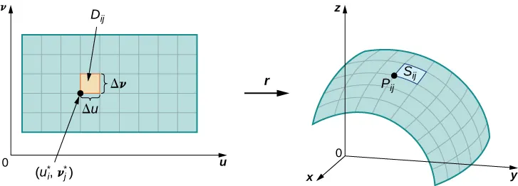
Let [latex]S[/latex] be a surface with parameterization [latex]\mathbf{r}(u,v) = \langle x(u,v), y(u,v), z(u,v) \rangle[/latex] over some parameter domain [latex]D[/latex]. We assume the surface parameterization is continuously differentiable—meaning each component function has continuous partial derivatives. For simplicity, assume [latex]D[/latex] is a rectangle (this material extends to nonrectangular domains). Divide rectangle [latex]D[/latex] into subrectangles [latex]D_{ij}[/latex] with horizontal width [latex]\Delta u[/latex] and vertical length [latex]\Delta v[/latex].
Suppose [latex]i[/latex] ranges from [latex]1[/latex] to [latex]m[/latex] and [latex]j[/latex] ranges from [latex]1[/latex] to [latex]n[/latex], so [latex]D[/latex] is subdivided into [latex]mn[/latex] rectangles. This division of [latex]D[/latex] into subrectangles gives a corresponding division of surface [latex]S[/latex] into pieces [latex]S_{ij}[/latex]. Choose point [latex]P_{ij}[/latex] in each piece [latex]S_{ij}[/latex]. Point [latex]P_{ij}[/latex] corresponds to point [latex](u_i, v_j)[/latex] in the parameter domain.
Grid Curves and Tangent Vectors
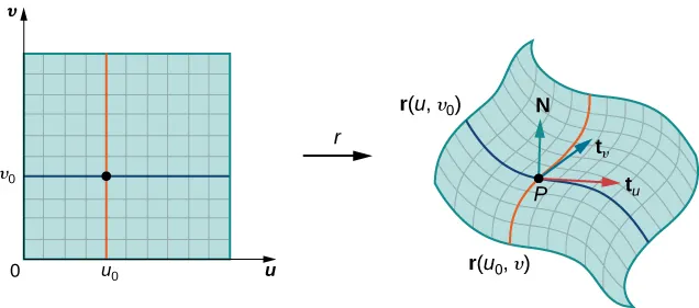
We can form a grid with lines parallel to the [latex]u[/latex]-axis and [latex]v[/latex]-axis in the [latex]uv[/latex]-plane. These grid lines correspond to a set of grid curves on surface [latex]S[/latex] that is parameterized by [latex]\mathbf{r}(u,v)[/latex].
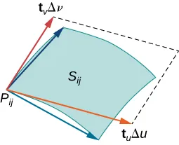
Without loss of generality, assume [latex]P_{ij}[/latex] is located at the corner of two grid curves, as in Figure 9. If we think of [latex]\mathbf{r}[/latex] as a mapping from the [latex]uv[/latex]-plane to [latex]\mathbb{R}^3[/latex], the grid curves are the image of the grid lines under [latex]\mathbf{r}[/latex].
Consider the grid lines through point [latex](u_i, v_j)[/latex]. One line is given by [latex]x = u_i[/latex], [latex]y = v[/latex]; the other is given by [latex]x = u[/latex], [latex]y = v_j[/latex]. In the first grid line, the horizontal component is held constant, yielding a vertical line through [latex](u_i, v_j)[/latex]. In the second grid line, the vertical component is held constant, yielding a horizontal line through [latex](u_i, v_j)[/latex]. The corresponding grid curves are [latex]\mathbf{r}(u_i, v)[/latex] and [latex]\mathbf{r}(u, v_j)[/latex], and these curves intersect at point [latex]P_{ij}[/latex].
Now consider the vectors that are tangent to these grid curves. For grid curve [latex]{\bf{r}}(u_i,v)[/latex] the tangent vector at [latex]P_{ij}[/latex] is:
[latex]{\bf{t}}_v(P_{ij})={\bf{r}}_v(u_i,v_j)=\langle{x}_v(u_i,v_j),y_v(u_i,v_j),z_v(u_i,v_j)\rangle[/latex].
For grid curve [latex]{\bf{r}}(u,v_j)[/latex], the tangent vector at [latex]P_{ij}[/latex] is:
[latex]{\bf{t}}_u(P_{ij})={\bf{r}}_y(u_i,v_j)=\langle{x}_v(u_i,v_j),y_u(u_i,v_j),z_u(u_i,v_j)\rangle[/latex].
If vector [latex]{\bf{N}}={\bf{t}}_u(P_{ij})\times{\bf{t}}_u(P_{ij}[/latex] exists and is not zero, then the tangent plane at [latex]P_{ij}[/latex] exists (Figure 10).
If piece [latex]S_{ij}[/latex] is small enough, then the tangent plane at point [latex]P_{ij}[/latex] is a good approximation of piece [latex]S_{ij}[/latex].
Approximating Surface Area
The tangent plane at [latex]P_{ij}[/latex] contains vectors [latex]\mathbf{t}_u(P_{ij})[/latex] and [latex]\mathbf{t}_v(P_{ij})[/latex]. Therefore, the parallelogram spanned by these two vectors lies in the tangent plane.
Since the original rectangle in the [latex]uv[/latex]-plane corresponding to [latex]S_{ij}[/latex] has width [latex]\Delta u[/latex] and length [latex]\Delta v[/latex], we approximate [latex]S_{ij}[/latex] using the parallelogram spanned by [latex]\Delta{u}{\bf{t}}_u(P_{ij})[/latex] and [latex]\Delta{v}{\bf{t}}_v(P_{ij})[/latex].
In other words, we scale the tangent vectors by the constants [latex]\Delta u[/latex] and [latex]\Delta v[/latex] to match the scale of the original division of rectangles in the parameter domain.
Therefore, the area of the parallelogram used to approximate the area of [latex]S_{ij}[/latex] is:
[latex]\Delta{S_{ij}}\approx||(\Delta{u}{\bf{t}}_u(P_{ij}))\times(\Delta{v}{\bf{t}}_v(P_{ij}))=||{\bf{t}}_u(P_{ij})\times{\bf{t}}_v(P_{ij})||\Delta{u}\Delta{v}[/latex].
Varying point [latex]P_{ij}[/latex] over all pieces [latex]S_{ij}[/latex] and the previous approximation leads to the following definition of surface area of a parametric surface (Figure 11).
surface area of a parametric surface
Let [latex]{\bf{r}}(u,v)=\langle(x(u,v),y(u,v),z(u,v)\rangle[/latex] with parameter domain [latex]D[/latex] be a smooth parameterization of surface [latex]S[/latex]. Furthermore, assume that [latex]S[/latex] is traced out only once as [latex](u, v)[/latex] varies over [latex]D[/latex]. The surface area of [latex]S[/latex] is:
[latex]\large{\displaystyle\iint_D||{\bf{t}}_u\times{\bf{t}}_v||dA}[/latex],
where [latex]{\bf{t}}_u=\left\langle\frac{\partial{x}}{\partial{u}},\frac{\partial{y}}{\partial{u}},\frac{\partial{z}}{\partial{u}}\right\rangle\text{ and }{\bf{t}}_v=\left\langle\frac{\partial{x}}{\partial{v}},\frac{\partial{y}}{\partial{v}},\frac{\partial{z}}{\partial{v}}\right\rangle[/latex].
Show that the surface area of the sphere [latex]x^{2}+y^{2}+z^{2}=r^{2}[/latex] is [latex]4\pi{r}^2[/latex].
Surfaces of Revolution
In addition to parameterizing surfaces given by equations or standard geometric shapes such as cones and spheres, we can also parameterize surfaces of revolution. This lets us calculate the surface area of a surface of revolution using the same techniques.
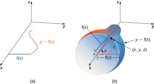
Let [latex]y = f(x) \geq 0[/latex] be a positive single-variable function on the domain [latex]a \leq x \leq b[/latex], and let [latex]S[/latex] be the surface obtained by rotating [latex]f[/latex] about the [latex]x[/latex]-axis (Figure 13). Let [latex]\theta[/latex] be the angle of rotation. Then [latex]S[/latex] can be parameterized with parameters [latex]x[/latex] and [latex]\theta[/latex] by:
[latex]\mathbf{r}(x,\theta) = \langle x, f(x)\cos\theta, f(x)\sin\theta \rangle, \quad a \leq x \leq b, \quad 0 \leq \theta \leq 2\pi[/latex]