We can represent a vector field using component functions or unit vectors, but visualizing it requires a different approach. The challenge is that a vector field in [latex]\mathbb{R}^2[/latex] has both its domain and range in [latex]\mathbb{R}^2[/latex], which means a complete “graph” would require four-dimensional space. Since we can’t visualize four dimensions, we use a clever alternative.
To draw a vector field in [latex]\mathbb{R}^2[/latex], we draw the vector associated with each point at that point’s location in the plane. For example, if point [latex](4, -1)[/latex] has the associated vector [latex]\langle 3,1 \rangle[/latex], we draw vector [latex]\langle 3,1 \rangle[/latex] starting at point [latex](4,-1)[/latex].
We should plot enough vectors to see the general shape, but not so many that the sketch becomes cluttered. If you plotted a vector at every single point, the entire region would be filled and the pattern would be impossible to see.
Choose points at grid line intersections and plot several representative vectors from each quadrant.
Two Important Types of Vector Fields
This module focuses on two types of vector fields in [latex]\mathbb{R}^2[/latex]: radial fields and rotational fields.
Radial fields model gravitational fields and energy source fields. In a radial field:
All vectors either point directly toward or directly away from the origin
The magnitude of any vector depends only on its distance from the origin
The vector at point [latex](x, y)[/latex] is perpendicular to the circle centered at the origin containing [latex](x, y)[/latex
All vectors on the same circle have the same magnitude
Rotational fields model the movement of fluid in a vortex. In a rotational field:
The vector at point [latex](x, y)[/latex] is tangent (not perpendicular) to a circle with radius [latex]r = \sqrt{x^2 + y^2}[/latex]
All vectors point either clockwise or counterclockwise
The magnitude of a vector depends only on its distance from the origin
Sketch the vector field [latex]{\bf{F}}(x,y)=\frac{x}2{\bf{i}}+\frac{y}2{\bf{j}}[/latex].
To sketch this vector field, choose a sample of points from each quadrant and compute the corresponding vector. The following table gives a representative sample of points in a plane and the corresponding vectors.
[latex](x, y)[/latex]
[latex]F(x, y)[/latex]
[latex](x, y)[/latex]
[latex]F(x, y)[/latex]
[latex](x, y)[/latex]
[latex]F(x, y)[/latex]
[latex](1, 0)[/latex]
[latex]\langle\frac12,0\rangle[/latex]
[latex](2, 0)[/latex]
[latex]\langle1,0\rangle[/latex]
[latex](1, 1)[/latex]
[latex]\langle\frac12,\frac12\rangle[/latex]
[latex](0, 1)[/latex]
[latex]\langle0,\frac12\rangle[/latex]
[latex](0, 2)[/latex]
[latex]\langle0,1\rangle[/latex]
[latex](-1, 1)[/latex]
[latex]\langle-\frac12,\frac12\rangle[/latex]
[latex](-1, 0)[/latex]
[latex]\langle-\frac12,0\rangle[/latex]
[latex](-2, 0)[/latex]
[latex]\langle-1,0\rangle[/latex]
[latex](-1, -1)[/latex]
[latex]\langle-\frac12,-\frac12\rangle[/latex]
[latex](0, -1)[/latex]
[latex]\langle0,-\frac12\rangle[/latex]
[latex](0, -2)[/latex]
[latex]\langle0,-1\rangle[/latex]
[latex](1, -1)[/latex]
[latex]\langle\frac12,-\frac12\rangle[/latex]
Figure 2(a) shows the vector field. To see that each vector is perpendicular to the corresponding circle, Figure 2(b) shows circles overlain on the vector field.
Figure 2. (a) A visual representation of the radial vector field [latex]\small{{\bf{F}}(x,y)=\frac{x}2{\bf{i}}+\frac{y}2{\bf{j}}}[/latex]. (b) The radial vector field [latex]\small{{\bf{F}}(x,y)=\frac{x}2{\bf{i}}+\frac{y}2{\bf{j}}}[/latex] with overlaid circles. Notice that each vector is perpendicular to the circle on which it is located.
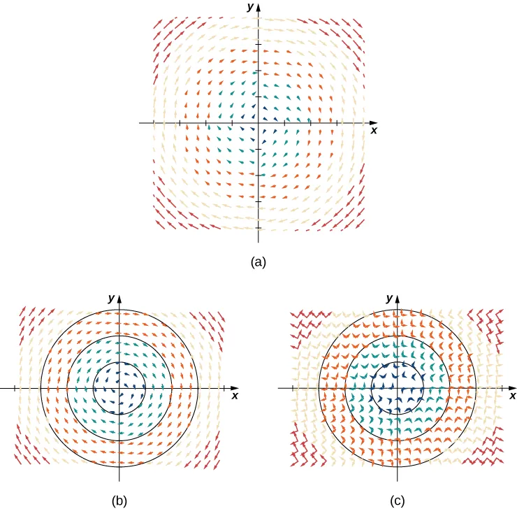
Sketch the vector field [latex]{\bf{F}}(x,y)=\langle{y},-x\rangle[/latex].
Create a table (see the one that follows) using a representative sample of points in a plane and their corresponding vectors. Figure 5 shows the resulting vector field.
[latex](x, y)[/latex]
[latex]F(x, y)[/latex]
[latex](x, y)[/latex]
[latex]F(x, y)[/latex]
[latex](x, y)[/latex]
[latex]F(x, y)[/latex]
[latex](1, 0)[/latex]
[latex]\langle0,-1\rangle[/latex]
[latex](2, 0)[/latex]
[latex]\langle0,-2\rangle[/latex]
[latex](1, 1)[/latex]
[latex]\langle1,-1\rangle[/latex]
[latex](0, 1)[/latex]
[latex]\langle1,0\rangle[/latex]
[latex](0, 2)[/latex]
[latex]\langle2,0\rangle[/latex]
[latex](-1, 1)[/latex]
[latex]\langle1,1\rangle[/latex]
[latex](-1, 0)[/latex]
[latex]\langle0,1\rangle[/latex]
[latex](-2, 0)[/latex]
[latex]\langle0,2\rangle[/latex]
[latex](-1, -1)[/latex]
[latex]\langle-1,1\rangle[/latex]
[latex](0, -1)[/latex]
[latex]\langle-1,0\rangle[/latex]
[latex](0, -2)[/latex]
[latex]\langle-2,0\rangle[/latex]
[latex](1, -1)[/latex]
[latex]\langle-1,-1\rangle[/latex]
Figure 6.5 (a) A visual representation of vector field F(x,y)=⟨y,−x⟩. (b) Vector field F(x,y)=⟨y,−x⟩ with circles centered at the origin. (c) Vector F(a,b) is perpendicular to radial vector ⟨a,b⟩ at point (a,b).
Analysis
Note that vector [latex]{\bf{F}}(a,b)=\langle{b},-a\rangle[/latex] points clockwise and is perpendicular to radial vector [latex]\langle{a},b\rangle[/latex]. (We can verify this assertion by computing the dot product of the two vectors:[latex]\langle{a},b\rangle\cdot\langle{-b},a\rangle=-ab+ab=0[/latex].) Furthermore, vector [latex]\langle{b},-a\rangle[/latex] has length [latex]r=\sqrt{a^2+b^2}[/latex]. Thus, we have a complete description of this rotational vector field: the vector associated with point [latex](a, b)[/latex] is the vector with length [latex]r[/latex] tangent to the circle with radius [latex]r[/latex], and it points in the clockwise direction.
Rotational vector fields are used to analyze major storm systems, including hurricanes and cyclones. An interesting pattern emerges:
In the northern hemisphere, storms rotate counterclockwise
In the southern hemisphere, storms rotate clockwise
This effect is caused by Earth's rotation about its axis and is called the Coriolis Effect.
Sketch vector field [latex]{\bf{F}}(x,y)=\frac{y}{x^2+y^2}{\bf{i}}-\frac{x}{x^2+y^2}{\bf{j}}[/latex].
To visualize this vector field, first note that the dot product [latex]{\bf{F}}(a,b)\cdot(a{\bf{i}}+b{\bf{j}})[/latex] is zero for any point [latex](a,b)[/latex]. Therefore, each vector is tangent to the circle on which it is located. Also, as [latex](a,b)\to(0,0)[/latex], the magnitude of [latex]{\bf{F}}(a,b)[/latex] goes to infinity. To see this, note that
Since [latex]\frac1{a^2+b^2}\to\infty[/latex] as [latex](a,b)\to(0,0)[/latex] then [latex]||{\bf{F}}(a,b)||\to\infty[/latex] as [latex](a,b)\to(0,0)[/latex]. This vector field looks similar to the vector field in Example "Chapter Opener: Drawing a Rotational Vector Field", but in this case the magnitudes of the vectors close to the origin are large. The table below shows a sample of points and the corresponding vectors, and Figure 6 shows the vector field. Note that this vector field models the whirlpool motion of the river in Figure 1(b). The domain of this vector field is all of [latex]\mathbb{R}^2[/latex] except for point [latex](0, 0)[/latex].
[latex](x, y)[/latex]
[latex]F(x, y)[/latex]
[latex](x, y)[/latex]
[latex]F(x, y)[/latex]
[latex](x, y)[/latex]
[latex]F(x, y)[/latex]
[latex](1, 0)[/latex]
[latex]\langle0,-1\rangle[/latex]
[latex](2, 0)[/latex]
[latex]\langle0,-\frac12\rangle[/latex]
[latex](1, 1)[/latex]
[latex]\langle\frac12,-\frac12\rangle[/latex]
[latex](0, 1)[/latex]
[latex]\langle1,0\rangle[/latex]
[latex](0, 2)[/latex]
[latex]\langle\frac12,0\rangle[/latex]
[latex](-1, 1)[/latex]
[latex]\langle\frac12,\frac12\rangle[/latex]
[latex](-1, 0)[/latex]
[latex]\langle0,1\rangle[/latex]
[latex](-2, 0)[/latex]
[latex]\langle0,\frac12\rangle[/latex]
[latex](-1, -1)[/latex]
[latex]\langle-\frac12,\frac12\rangle[/latex]
[latex](0, -1)[/latex]
[latex]\langle-1,0\rangle[/latex]
[latex](0, -2)[/latex]
[latex]\langle-\frac12,0\rangle[/latex]
[latex](1, -1)[/latex]
[latex]\langle-\frac12,-\frac12\rangle[/latex]
Figure 6. A visual representation of vector field [latex]\small{{\bf{F}}(x,y)=\frac{y}{x^2+y^2}{\bf{i}}-\frac{x}{x^2+y^2}{\bf{j}}}[/latex]. This vector field could be used to model whirlpool motion of a fluid.
Suppose that [latex]{\bf{v}}(x,y)=-\frac{2y}{x^2+y^2}{\bf{i}}+\frac{2x}{x^2+y^2}{\bf{j}}[/latex] is the velocity field of a fluid. How fast is the fluid moving at point [latex](1, -1)[/latex]?(Assume the units of speed are meters per second.)
To find the velocity of the fluid at point [latex](1, -1)[/latex], substitute the point into [latex]\bf{v}[/latex]:
The speed of the fluid at [latex](1, -1)[/latex] is the magnitude of this vector. Therefore, the speed is [latex]||{\bf{i}}+{\bf{j}}||=\sqrt2[/latex] m/sec.
Unit Vector Fields
A vector field [latex]\mathbf{F}[/latex] is a unit vector field if the magnitude of each vector in the field is [latex]1[/latex]. In a unit vector field, only the direction of each vector matters—not its magnitude.
unit vector field
A vector field [latex]\mathbf{F}[/latex] is a unit vector field if [latex]||\mathbf{F}(x,y)|| = 1[/latex] for all points [latex](x, y)[/latex] in the domain.
Show that vector field [latex]{\bf{F}}(x,y)=\left\langle\frac{y}{\sqrt{x^2+y^2}},-\frac{x}{\sqrt{x^2+y^2}}\right\rangle[/latex] is a unit vector field.
To show that [latex]\bf{F}[/latex] is a unit field, we must show that the magnitude of each vector is [latex]1[/latex]. Note that
Therefore, [latex]\bf{F}[/latex] is a unit vector field.
Unit vector fields are particularly useful when studying fluid flow where we care only about the direction of flow at each point, not the speed. When speed is irrelevant and only direction matters, the unit vector field associated with velocity is what we study.
Normalizing a Vector Field
If [latex]\mathbf{F}(x,y) = \langle P, Q, R \rangle[/latex] is a vector field, the corresponding unit vector field is:
The process of dividing [latex]\mathbf{F}[/latex] by its magnitude to form the unit vector field [latex]\mathbf{F}/||\mathbf{F}||[/latex] is called normalizing the field [latex]\mathbf{F}[/latex].
You've normalized individual vectors before by dividing by their magnitude. Normalizing a vector field applies the same idea to every vector in the field simultaneously:
For vector [latex]\mathbf{v}[/latex], the unit vector is [latex]\frac{\mathbf{v}}{||\mathbf{v}||}[/latex]
For vector field [latex]\mathbf{F}[/latex], the unit vector field is [latex]\frac{\mathbf{F}}{||\mathbf{F}||}[/latex]
Vector Fields in [latex]\mathbb{R}^3[/latex]
Vector fields in three dimensions can model gravitational or electromagnetic fields, fluid flow, or heat flow throughout three-dimensional space. While a two-dimensional vector field might model water flow on a river's surface, a three-dimensional field can model the flow throughout the entire depth of the river.
The extra dimension makes vector fields in [latex]\mathbb{R}^3[/latex] more challenging to visualize, but the idea remains the same: plot enough vectors to show the overall shape. We can use a similar method to visualizing fields in [latex]\mathbb{R}^2[/latex] by choosing representative points in each octant.
Just as with vector fields in [latex]\mathbb{R}^2[/latex], we represent vector fields in [latex]\mathbb{R}^3[/latex] using component functions. We need an extra component function for the extra dimension.
When sketching a vector field in [latex]\mathbb{R}^3[/latex]:
Start by understanding the field's behavior in coordinate planes ([latex]xy[/latex]-plane, [latex]xz[/latex]-plane, [latex]yz[/latex]-plane)
Consider how the vectors change as you move perpendicular to these planes
Look for symmetry that can simplify your understanding
Plot representative vectors from different octants
Describe vector field [latex]{\bf{F}}(x,y,z)=\langle1,1,z\rangle[/latex].
For this vector field, the [latex]x[/latex] and [latex]y[/latex] components are constant, so every point in [latex]\mathbb{R}^3[/latex] has an associated vector with [latex]x[/latex] and [latex]y[/latex] components equal to one. To visualize [latex]\bf{F}[/latex], we first consider what the field looks like in the [latex]xy[/latex]-plane. In the [latex]xy[/latex]-plane, [latex]z=0[/latex]. Hence, each point of the form [latex](a, b, 0)[/latex] has vector [latex]\langle 1,1,0\rangle[/latex] associated with it. For points not in the [latex]xy[/latex]-plane but slightly above it, the associated vector has a small but positive [latex]z[/latex] component, and therefore the associated vector points slightly upward. For points that are far above the [latex]xy[/latex]-plane, the [latex]z[/latex] component is large, so the vector is almost vertical. Figure 8 shows this vector field.
Figure 8. A visual representation of vector field [latex]{\bf{F}}(x,y,z)=\langle1,1,z\rangle[/latex].