Introduction to Partial Derivatives: Learn It 1

Giselle Miller

Introduction to Partial Derivatives: Learn It 1

Calculate the partial derivatives of a function of two variables
Calculate the partial derivatives of a function of more than two variables
Find higher-order partial derivatives of a function of two variables

Derivatives of a Function of Two Variables

In single-variable calculus, the derivative represents an instantaneous rate of change of [latex]y[/latex] with respect to [latex]x[/latex]. We write this using Leibniz notation as [latex]dy/dx[/latex], where [latex]y[/latex] is the dependent variable and [latex]x[/latex] is the independent variable.

For a function [latex]z=f(x,y)[/latex] of two variables, both [latex]x[/latex] and [latex]y[/latex] are independent variables and [latex]z[/latex] is the dependent variable. This immediately raises two questions: How do we adapt Leibniz notation for two variables? What does the derivative even mean when we have two inputs? The answer lies in partial derivatives.

partial derivatives

Let [latex]f(x, y)[/latex] be a function fo two variables.

[latex]\\[/latex]

The partial derivative of [latex]f[/latex] with respect to [latex]x[/latex], written as [latex]\frac{\partial f}{\partial x}[/latex] or [latex]f_x[/latex], is defined as

[latex]\dfrac{\partial f}{\partial x}=\underset{h\to 0}{\text{lim}}\dfrac{f(x+h,y)-f(x,y)}{h}[/latex].

The partial derivative of [latex]f[/latex] with respect to [latex]y[/latex], written as [latex]\frac{\partial f}{\partial y}[/latex] or [latex]f_y[/latex], is defined as

[latex]\dfrac{\partial f}{\partial y}=\underset{k\to 0}{\text{lim}}\dfrac{f(x,y+k)-f(x,y)}{k}[/latex].

This definition reveals two key differences from single-variable derivatives. First, the notation changes—we use the symbol [latex]\partial[/latex] instead of [latex]d[/latex]. This rounded “[latex]d[/latex]” is called “partial,” so [latex]\partial f/\partial x[/latex] is read as “the partial of [latex]f[/latex] with respect to [latex]x[/latex].”

Second, we now have two different derivatives we can compute, one with respect to each independent variable. Depending on which variable we choose, we get entirely different partial derivatives.

Use the definition of the partial derivative as a limit to calculate [latex]\partial f/\partial x[/latex] and [latex]\partial f/\partial y[/latex] for the function

[latex]f(x, y)=x^{2}-3xy+2y^{2}-4x+5y-12[/latex].

First, calculate [latex]f(x+h, y)[/latex].

[latex]\begin{array}{ccc}\hfill {f(x+h, y)} & =\hfill & {(x+h)^{2}-3(x+h)y+2y^{2}-4(x+h)+5y-12} \hfill \\ \hfill & =\hfill & {x^{2}+2xh+h^{2}-3xy-3hy+2y^{2}-4x-4h+5y-12.} \hfill \\ \hfill \end{array}[/latex]

Next, substitute this into our definition and simplify:

[latex]\begin{array}{ccc}\hfill {\frac{\partial f}{\partial x}} & =\hfill & {\displaystyle\lim_{h\to 0}\frac{f(x+h, y)-f(x, y)}{h}} \hfill \\ \hfill & =\hfill & {\displaystyle\lim_{h\to 0}\frac{(x^{2}+2xh+h^{2}-3xy-3hy+2y^{2}-4x-4h+5y-12)-(x^{2}-3xy+2y^{2}-4x+5y-12)}{h}} \hfill \\ \hfill & =\hfill & {\displaystyle\lim_{h\to 0}\frac{x^{2}+2xh+h^{2}-3xy-3hy+2y^{2}-4x-4h+5y-12-x^{2}+3xy-2y^{2}+4x-5y+12}{h}}\hfill \\ \hfill & =\hfill & {\displaystyle\lim_{h\to 0}\frac{2xh+h^{2}-3hy-4h}{h}}\hfill \\ \hfill & =\hfill & {\displaystyle\lim_{h\to 0}\frac{h(2x+h-3y-4)}{h}}\hfill \\ \hfill & =\hfill & {\displaystyle\lim_{h\to 0}(2x+h-3y-4)}\hfill \\ \hfill & =\hfill & {2x-3y-4}\hfill \\ \hfill \end{array}[/latex]

To calculate [latex]\frac{\partial f}{\partial y}[/latex], first calculate [latex]f(x, y+h)[/latex]:

[latex]\begin{array}{ccc}\hfill {f(x, y+h)} & =\hfill & {x^{2}-3x(y+h)+2(y+h)^{2}-4x+5(y+h)-12}\hfill \\ \hfill & =\hfill & {x^{2}-3xy-3xh+2y^{2}+4yh+2h^{2}-4x+5y+5h-12.}\hfill \\ \hfill \end{array}[/latex]

Next, substitute this into our definition and simplify:

[latex]\begin{array}{ccc}\hfill {\frac{\partial f}{\partial y}} & =\hfill & {\displaystyle\lim_{k\to 0}\frac{f(x, y+h)-f(x, y)}{k}}\hfill \\ \hfill & =\hfill & {\displaystyle\lim_{k\to 0}\frac{(x^{2}-3xy-3xh+2y^{2}+4yh+2h^{2}-4x+5y+5h-12)-(x^{2}-3xy+2y^{2}-4x+5y-12)}{k}}\hfill \\ \hfill & =\hfill & {\displaystyle\lim_{k\to 0}\frac{x^{2}-3xy-3xh+2y^{2}+4yh+2h^{2}-4x+5y+5h-12-x^{2}+3xy-2y^{2}+4x-5y+12}{k}}\hfill \\ \hfill & =\hfill & {\displaystyle\lim_{k\to 0}\frac{-3xk+4yk+2k^{2}+5k}{k}}\hfill \\ \hfill & =\hfill & {\displaystyle\lim_{k\to 0}\frac{h(-3x+4y+2k+5)}{k}}\hfill \\ \hfill & =\hfill & {\displaystyle\lim_{k\to 0}(-3x+4y+2k+5)}\hfill \\ \hfill & =\hfill & {-3x+4y+5.} \hfill \\ \hfill \end{array}[/latex]

Computing Partial Derivatives

The key idea when calculating partial derivatives is simple: treat all independent variables except the one you’re differentiating with respect to as constants. Then differentiate as you would with a single-variable function.

Why does this work? When we fix [latex]y[/latex] and define [latex]g(x)=f(x,y)[/latex] as a function of [latex]x[/latex] only, we get:

[latex]g'(x)=\underset{h\to 0}{\text{lim}}\dfrac{g(x+h)-g(x)}{h}=\underset{h\to 0}{\text{lim}}\dfrac{f(x+h,y)-f(x,y)}{h}=\dfrac{\partial f}{\partial x}[/latex].

The same reasoning applies for the partial derivative with respect to [latex]y[/latex]. Fix [latex]x[/latex] and define [latex]h(y)=f(x,y)[/latex] as a function of [latex]y[/latex] only:

[latex]h'(y)=\underset{k\to 0}{\text{lim}}\dfrac{h(y+k)-h(y)}{k}=\underset{k\to 0}{\text{lim}}\dfrac{f(x,y+k)-f(x,y)}{k}=\dfrac{\partial f}{\partial y}[/latex].

All the differentiation rules you learned in single-variable calculus still apply.

To find [latex]\dfrac{\partial f}{\partial x}[/latex]: Treat [latex]y[/latex] as a constant and differentiate with respect to [latex]x[/latex].

To find [latex]\dfrac{\partial f}{\partial y}[/latex]: Treat [latex]x[/latex] as a constant and differentiate with respect to [latex]y[/latex].

Calculate [latex]\partial f/\partial x[/latex] and [latex]\partial f/\partial y[/latex] for the following functions by holding the opposite variable constant then differentiating:

[latex]f(x, y)=x^{2}-3xy+2y^{2}-4x+5y-12[/latex].
[latex]g(x, y)=\sin{(x^{2}y-2x+4)}[/latex]

To calculate [latex]\partial f/\partial x[/latex], treat the variable [latex]y[/latex] as a constant. Then differentiate [latex]f(x, y)[/latex] with respect to [latex]x[/latex] using the sum, difference, and power rules:
[latex]\begin{array}{ccc}\hfill {\frac{\partial f}{\partial x}} & =\hfill & {\frac{\partial}{\partial x}\big[x^{2}-3xy+2y^{2}-4x+5y-12\big]}\hfill \\ \hfill & =\hfill & {\frac{\partial}{\partial x}\big[x^{2}\big]-\frac{\partial}{\partial x}\big[3xy\big]+\frac{\partial}{\partial x}\big[2y^{2}\big]-\frac{\partial}{\partial x}\big[4x\big]+\frac{\partial}{\partial x}\big[5y\big]-\frac{\partial}{\partial x}\big[12\big]}\hfill \\ \hfill & =\hfill & {2x-3y+0-4+0-0}\hfill \\ \hfill & =\hfill & {2x-3y-4.} \hfill \\ \hfill \end{array}[/latex]

The derivatives of the third, fifth, and sixth terms are all zero because they do not contain the variable [latex]x[/latex], so they are treated as constant terms. The derivative of the second term is equal to the coefficient of [latex]x[/latex], which is [latex]-3y[/latex]. Calculating [latex]\partial f/\partial y[/latex]:

[latex]\begin{array}{ccc}\hfill {\frac{\partial f}{\partial y}} & =\hfill & {\frac{\partial}{\partial y}\big[x^{2}-3xy+2y^{2}-4x+5y-12\big]}\hfill \\ \hfill & =\hfill & {\frac{\partial}{\partial y}\big[x^{2}\big]-\frac{\partial}{\partial y}\big[3xy\big]+\frac{\partial}{\partial y}\big[2y^{2}\big]-\frac{\partial}{\partial y}\big[4x\big]+\frac{\partial}{\partial y}\big[5y\big]-\frac{\partial}{\partial y}\big[12\big]}\hfill \\ \hfill & =\hfill & {-3x+4y-0+5-0}\hfill \\ \hfill & =\hfill & {-3x+4y+5.} \hfill \\ \hfill \end{array}[/latex]

These are the same answers obtained in the previous example
To calculate [latex]\partial g/\partial x[/latex], create the variable [latex]y[/latex] as a constant. Then differentiate [latex]g(x, y)[/latex] with respect to [latex]x[/latex] using the chain rule and power rule:
[latex]\begin{array}{ccc}\hfill{\frac{\partial g}{\partial y}} & =\hfill & {\frac{\partial}{\partial x}\big[\sin{(x^{2}y-2x+4)}\big]} \hfill \\ \hfill & =\hfill & {\cos{(x^{2}y-2x+4)}\frac{\partial}{\partial x}[x^{2}y-2x+4]}\hfill \\ \hfill & =\hfill & {(2xy-2)\cos{(x^{2}y-2x+4)}.}\hfill \\ \hfill \end{array}[/latex]

To calculate [latex]\partial f/\partial y[/latex], treat the variable [latex]x[/latex] as a constant. Then differentiate [latex]g(x, y)[/latex] with respect to [latex]y[/latex] using the chain rule and power rule:

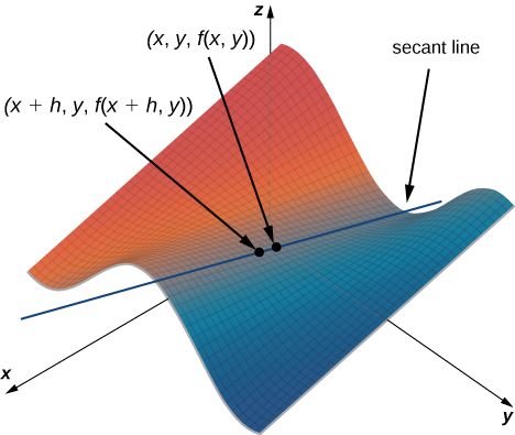
[latex]\begin{array}{ccc}\hfill {\frac{\partial g}{\partial y}} & =\hfill & {\frac{\partial}{\partial y}\big[\sin{(x^{2}y-2x+4)}\big]}\hfill \\ \hfill & =\hfill & {\cos{(x^{2}y-2x+4)}\frac{\partial}{\partial x}[x^{2}y-2x+4]} \hfill \\ \hfill & =\hfill & {x^{2}\cos{(x^{2}-2x+4)}.}\hfill \\ \hfill \end{array}[/latex]

Geometric Interpretation

How should we interpret partial derivatives geometrically? Recall that the graph of a function of two variables is a surface in [latex]\mathbb{R}^{3}[/latex]. If we remove the limit from the definition of the partial derivative with respect to [latex]x[/latex], we’re left with the difference quotient:

[latex]\dfrac{f(x+h,y)-f(x,y)}{h}[/latex].

This looks just like the difference quotient for a single-variable derivative, except [latex]y[/latex] is along for the ride as a constant. Figure 1 shows a surface described by [latex]z=f(x,y)[/latex].

A complicated curve in xyz space with a secant line through the points (x, y, f(x, y)) and (x + h, y, f(x + h, y)). — Figure 1. Secant line passing through the points [latex]\small{(x,y,f(x,y))}[/latex] and [latex]\small{(x+h,y,f(x+h,y))}[/latex].

In Figure 1, [latex]h[/latex] is positive. When we graph the points [latex]f(x, y)[/latex] and [latex]f(x+h, y)[/latex], the slope of the secant line connecting them is:

[latex]\dfrac{f(x+h,y)-f(x,y)}{h}[/latex].

This secant line runs parallel to the [latex]x[/latex]-axis. The slope represents an average rate of change of [latex]f[/latex] as we move parallel to the [latex]x[/latex]-axis. As [latex]h[/latex] approaches zero, the secant line’s slope approaches the tangent line’s slope.

If we instead change [latex]y[/latex] by an increment [latex]h[/latex] (while holding [latex]x[/latex] fixed), the secant line—and resulting tangent line—would be parallel to the [latex]y[/latex]-axis.

Therefore:

[latex]\dfrac{\partial f}{\partial x}[/latex] gives the slope of the tangent line to the surface parallel to the [latex]x[/latex]-axis at the point [latex](x, y, f(x, y))[/latex]
[latex]\dfrac{\partial f}{\partial y}[/latex] gives the slope of the tangent line to the surface parallel to the [latex]y[/latex]-axis at the point [latex](x, y, f(x, y))[/latex]

Think of partial derivatives as slopes in specific directions:

[latex]\dfrac{\partial f}{\partial x}[/latex]: slope when moving parallel to the [latex]x[/latex]-axis
[latex]\dfrac{\partial f}{\partial y}[/latex]: slope when moving parallel to the [latex]y[/latex]-axis

What about slopes in other directions? We’ll need directional derivatives for that, which we’ll discuss later.

You can also estimate partial derivatives using contour maps.

Use a contour map to estimate [latex]\partial g/\partial x[/latex] at the point [latex](\sqrt{5}, 0)[/latex] for the function

[latex]g(x, y)=\sqrt{9-x^{2}-y^{2}}[/latex].

The following graph represents a contour map for the function [latex]g(x, y)=\sqrt{9-x^{2}-y^{2}}[/latex].

A series of concentric circles with the center the origin. The first is marked c = 0 and has radius 3; the second is marked c = 1 and has radius slightly less than 3; and the third is marked c = 2 and has radius slightly more than 2. The graph is marked with the equation g(x, y) = the square root of the quantity (9 – x2 – y2). — Figure 2. Contour map for the function [latex]\small{g(x,y)=\sqrt{9-x^{2}-y^{2}}}[/latex], using [latex]\small{c=0,1,2}[/latex], and [latex]\small{3}[/latex] ([latex]\small{c=3}[/latex] corresponds to the origin).

The inner circle on the contour map corresponds to [latex]c=2[/latex] and the next circle out corresponds to [latex]c=1[/latex]. The first circle is given by the equation [latex]2=\sqrt{9-x^{2}-y^{2}}[/latex]; the second circle is given by the equation [latex]1=\sqrt{9-x^{2}-y^{2}}[/latex]. The first equation simplifies to [latex]x^{2}+y^{2}=5[/latex] and the second equation simplifies to [latex]x^{2}+y^{2}=8[/latex]. The [latex]x[/latex]-intercept of the first circle is [latex](\sqrt{5}, 0)[/latex] and the [latex]x[/latex]-intercept of the second circle is [latex](2\sqrt{2}, 0)[/latex]. We can estimate the value of [latex]\partial g/\partial x[/latex] evaluated at the point [latex](\sqrt{5}, 0)[/latex] using the slope formula:

[latex]\large{\frac{\partial g}{\partial x}\bigg|_{(x, y)=(\sqrt{5}, 0)}\approx\frac{g(\sqrt{5}, 0)-g(2\sqrt{2}, 0)}{\sqrt{5}-2\sqrt{2}}=\frac{2-1}{\sqrt{5}-2\sqrt{2}}=\frac{1}{\sqrt{5}-2\sqrt{2}}\approx -1.688.}[/latex]

To calculate the exact value of [latex]\partial g/\partial x[/latex] evaluated at the point [latex](\sqrt{5}, 0)[/latex], we start by finding [latex]\partial g/\partial x[/latex] using the chain rule. First, we rewrite the function as [latex]g(x, y)=\sqrt{9-x^{2}-y^{2}}=(9-x^{2}-y^{2})^{\frac{1}{2}}[/latex] and then differentiate with respect to [latex]x[/latex] while holding [latex]y[/latex] constant:

[latex]\large{\frac{\partial g}{\partial x}=\frac{1}{2}(9-x^{2}-y^{2})^{-\frac{1}{2}}(-2x)=-\frac{x}{\sqrt{9-x^{2}-y^{2}}}.}[/latex]

Next, we evaluate this expression using [latex]x=\sqrt{5}[/latex] and [latex]y=0[/latex]:

[latex]\large{\frac{\partial g}{\partial x}\bigg|_{(x, y)=(\sqrt{5}, 0)}=-\frac{\sqrt{5}}{\sqrt{9-(\sqrt{5})^{2}-(0)^{2}}}=-\frac{\sqrt{5}}{\sqrt{4}}=-\frac{\sqrt{5}}{2}\approx -1.118.}[/latex]

The estimate for the partial derivative corresponds to the slope of the secant line passing through the points [latex](\sqrt{5}, 0, g(\sqrt{5}, 0))[/latex] and [latex](2\sqrt{2}, 0, g(2\sqrt{2}, 0))[/latex]. It represents an approximation to the slope of the tangent line to the surface through the point [latex](\sqrt{5}, 0, g(\sqrt{5}, 0))[/latex], which is parallel to the [latex]x[/latex]-axis.