Circulation Form of Green’s Theorem
The first form of Green’s theorem that we examine is the circulation form. This form relates the vector line integral over a simple, closed plane curve [latex]C[/latex] to a double integral over the region enclosed by [latex]C[/latex]. Therefore, the circulation of a vector field along a simple closed curve can be transformed into a double integral and vice versa.
Green’s theorem, circulation form
Let [latex]D[/latex] be an open, simply connected region with a boundary curve [latex]C[/latex] that is a piecewise smooth, simple closed curve oriented counterclockwise (Figure 2). Let [latex]{\bf{F}}=\langle{P},Q\rangle[/latex] be a vector field with component functions that have continuous partial derivatives on [latex]D[/latex]. Then,
[latex]\displaystyle\oint_C{\bf{F}}\cdot{d}{\bf{r}}=\displaystyle\oint_CPdx+Qdy=\displaystyle\iint_D(Q_x-P_y)dA[/latex].
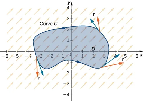
The proof of Green’s theorem is rather technical, and beyond the scope of this text. Here we examine a proof of the theorem in the special case that [latex]D[/latex] is a rectangle. For now, notice that we can quickly confirm that the theorem is true for the special case in which [latex]{\bf{F}}\langle{P},Q\rangle[/latex] is conservative. In this case,
[latex]\large{\displaystyle\oint_CPdx+Qdy=0}[/latex]
because the circulation is zero in conservative vector fields. By the cross-partial property of conservative fields theorem, [latex]{\bf{F}}[/latex] satisfies the cross-partial condition, so [latex]P_y=Q_x[/latex]. Therefore,
[latex]\large{\displaystyle\iint_D(Q_x-P_y)dA=\displaystyle\iint_D0dA=0=\displaystyle\oint_CPdx+Qdy}[/latex],
which confirms Green’s theorem in the case of conservative vector fields.
Proof
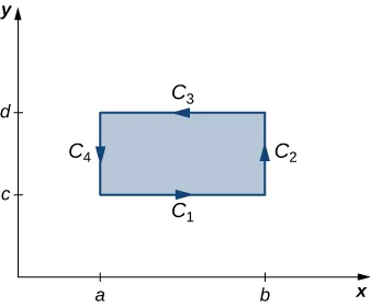
Let’s now prove that the circulation form of Green’s theorem is true when the region [latex]D[/latex] is a rectangle. Let [latex]D[/latex] be the rectangle [latex][a,b]\times[c,d][/latex] oriented counterclockwise. Then, the boundary [latex]C[/latex] of [latex]D[/latex] consists of four piecewise smooth pieces [latex]C_1[/latex], [latex]C_2[/latex], [latex]C_3[/latex], and [latex]C_4[/latex] (Figure 3). We parameterize each side of [latex]D[/latex] as follows:
[latex]\begin{aligned} C_1:{\bf{r}}_1(t)&=\langle{t},c\rangle,a\leq{t}\leq{b} \\ C_2:{\bf{r}}_2(t)&=\langle{b},t\rangle,c\leq{t}\leq{d} \\ -C_3:{\bf{r}}_3(t)&=\langle{t},d\rangle,a\leq{t}\leq{b} \\ -C_4:{\bf{r}}_4(t)&=\langle{a},t\rangle,c\leq{t}\leq{d} \end{aligned}[/latex].
Then,
[latex]\begin{aligned} \displaystyle\int_C{\bf{F}}\bullet{d}{\bf{r}}&=\displaystyle\int_{C_1}{\bf{F}}\bullet{d}{\bf{r}}+\displaystyle\int_{C_2}{\bf{F}}\bullet{d}{\bf{r}}+\displaystyle\int_{C_3}{\bf{F}}\bullet{d}{\bf{r}}+\displaystyle\int_{C_4}{\bf{F}}\bullet{d}{\bf{r}} \\ &=\displaystyle\int_{C_1}{\bf{F}}\bullet{d}{\bf{r}}+\displaystyle\int_{C_2}{\bf{F}}\bullet{d}{\bf{r}}-\displaystyle\int_{-C_3}{\bf{F}}\bullet{d}{\bf{r}}-\displaystyle\int_{-C_4}{\bf{F}}\bullet{d}{\bf{r}} \\ &=\displaystyle\int_a^b{\bf{F}}({\bf{r}}_1(t))\bullet{\bf{r}}_1(t)dt+\displaystyle\int_c^d{\bf{F}}({\bf{r}}_2(t))\bullet{\bf{r}}_2(t)dt-\displaystyle\int_a^b{\bf{F}}({\bf{r}}_3(t))\bullet{\bf{r}}_3(t)dt-\displaystyle\int_c^d{\bf{F}}({\bf{r}}_4(t))\bullet{\bf{r}}_4(t)dt \\ &=\displaystyle\int_a^bP(t,c)dt+\displaystyle\int_c^dQ(b,t)dt-\displaystyle\int_a^bP(t,d)dt-\displaystyle\int_c^dQ(a,t)dt \\ &=\displaystyle\int_a^b(P(t,c)-P(t,d))dt+\displaystyle\int_c^d(Q(b,t)-Q(a,t))dt \\ &=-\displaystyle\int_a^b(P(t,d)-P(t,c))dt+\displaystyle\int_c^d(Q(b,t)-Q(a,t))dt \end{aligned}[/latex].
By the Fundamental Theorem of Calculus,
[latex]\large{P(t,d)-P(t,c)=\displaystyle\int_c^d\frac{\partial}{\partial{y}}P(t,y)dy\text{ and }Q(b,t)-Q(a,t)=\displaystyle\int_a^b\frac{\partial}{\partial{x}}Q(x,t)dx}[/latex].
Therefore,
[latex]\begin{aligned} &-\displaystyle\int_a^b(P(t,d)-P(t,c)dt+\displaystyle\int_c^d(Q(b,t)-Q(a,t))dt \\ &=-\displaystyle\int_a^b\displaystyle\int_c^d\frac{\partial}{\partial{y}}P(t,y)dydt+\displaystyle\int_c^d\displaystyle\int_a^b\frac{\partial}{\partial{x}}Q(x,t)dxdt \end{aligned}[/latex].
But,
[latex]\begin{aligned} -\displaystyle\int_a^b\displaystyle\int_c^d\frac{\partial}{\partial{y}}P(t,y)dydt+\displaystyle\int_c^d\displaystyle\int_a^b\frac{\partial}{\partial{x}}Q(x,t)dxdt&=-\displaystyle\int_a^b\displaystyle\int_c^d\frac{\partial}{\partial{y}}P(x,y)dydx+\displaystyle\int_c^d\displaystyle\int_a^b\frac{\partial}{\partial{x}}Q(x,t)dxdy \\ &=\displaystyle\int_a^b\displaystyle\int_c^d(Q_x-P_y)dydx \\ &=\displaystyle\int \ \displaystyle\int_D(Q_x-P_y)dA \end{aligned}[/latex].
Therefore, [latex]\displaystyle\int_C{\bf{F}}\bullet{d}{\bf{r}}=\int\int_D(Q_{x}-P_{y})dA[/latex] and we have proved Green’s theorem in the case of a rectangle.
To prove Green’s theorem over a general region [latex]D[/latex], we can decompose [latex]D[/latex] into many tiny rectangles and use the proof that the theorem works over rectangles. The details are technical, however, and beyond the scope of this text.
[latex]_\blacksquare[/latex]
Calculate the line integral
[latex]\displaystyle\oint_Cx^2ydx+(y-3)dy[/latex]
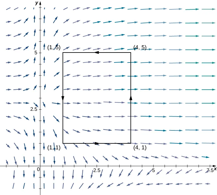
where [latex]C[/latex] is a rectangle with vertices [latex](1, 1)[/latex], [latex](4, 1)[/latex], [latex](4, 5)[/latex], and [latex](1, 5)[/latex] oriented counterclockwise.
Calculate the work done on a particle by force field
[latex]{\bf{F}}(x,y)=\langle{y}+\sin{x},e^y-x\rangle[/latex]
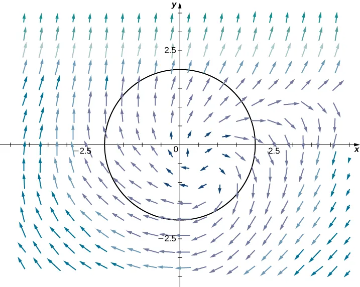
as the particle traverses circle [latex]x^2+y^2=4[/latex] exactly once in the counterclockwise direction, starting and ending at point [latex](2, 0)[/latex].
In the preceding two examples, the double integral in Green’s theorem was easier to calculate than the line integral, so we used the theorem to calculate the line integral. In the next example, the double integral is more difficult to calculate than the line integral, so we use Green’s theorem to translate a double integral into a line integral.
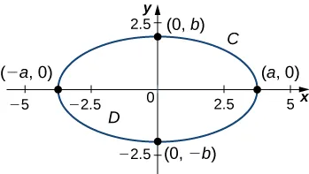
In the above example, we used vector field [latex]\mathbf{F}(x,y)=\langle P,Q\rangle=\left\langle-\frac{y}{2},\frac{x}{2}\right\rangle[/latex] to find the area of any ellipse. The logic of the previous example can be extended to derive a formula for the area of any region [latex]D[/latex]. Let [latex]D[/latex] be any region with a boundary that is a simple closed curve [latex]C[/latex] oriented counterclockwise. If [latex]\mathbf{F}(x,y)=\langle P,Q\rangle=\left\langle-\frac{y}{2},\frac{x}{2}\right\rangle[/latex], then by the same logic as in the previous example,
[latex]\text{area of }D=\displaystyle\iint_DdA=\frac12\displaystyle\oint_C-ydx+xdy[/latex].