Using Divergence and Curl
Now that we understand the basic concepts of divergence and curl, we can discuss their properties and establish relationships between them and conservative vector fields.
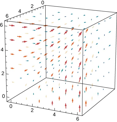
If [latex]\mathbf{F}[/latex] is a vector field in [latex]\mathbb{R}^3[/latex], then the curl of [latex]\mathbf{F}[/latex] is also a vector field in [latex]\mathbb{R}^3[/latex]. Therefore, we can take the divergence of a curl. The next theorem says that the result is always zero. This result is useful because it gives us a way to show that some vector fields are not the curl of any other field.
To give this result a physical interpretation, recall that divergence of a velocity field [latex]\mathbf{v}[/latex] at point [latex]P[/latex] measures the tendency of the corresponding fluid to flow out of [latex]P[/latex]. Since [latex]\text{div curl }(\mathbf{v})=0[/latex], the net rate of flow in vector field curl([latex]\mathbf{v}[/latex]) at any point is zero. Taking the curl of vector field [latex]\mathbf{F}[/latex] eliminates whatever divergence was present in [latex]\mathbf{F}[/latex].
divergence of the curl
Let [latex]{\bf{F}}=\langle{P},Q,R\rangle[/latex] be a vector field in [latex]\mathbb{R}^3[/latex] such that the component functions all have continuous second-order partial derivatives. Then,
Proof
By the definitions of divergence and curl, and by Clairaut’s theorem,
[latex]\begin{aligned} \text{div curl }({\bf{F}})&=\text{div }[(R_y-Q_z){\bf{i}}+(P_z-R_x){\bf{j}}+(Q_x-P_y){\bf{k}}] \\&=R_{yx}-Q_{xz}+P_{yz}-R_{yx}+Q_{zx}-P_{zy} \\ &=0 \end{aligned}[/latex].
[latex]_\blacksquare[/latex]
With the next two theorems, we show that if [latex]\mathbf{F}[/latex] is a conservative vector field then its curl is zero, and if the domain of [latex]\mathbf{F}[/latex] is simply connected then the converse is also true. This gives us another way to test whether a vector field is conservative.
curl of a conservative vector field
If [latex]{\bf{F}}=\langle{P},Q,R\rangle[/latex] is conservative, then [latex]\text{curl } \bf{F}=\bf{0}[/latex].
Proof
Since conservative vector fields satisfy the cross-partials property, all the cross-partials of [latex]{\bf{F}}[/latex] are equal. Therefore,
[latex]\begin{aligned} \text{curl }{\bf{F}}&=(R_y-Q_z){\bf{i}}+(P_z-R_x){\bf{j}}+(Q_x-P_y){\bf{k}} \\ &=0 \end{aligned}[/latex].
[latex]_\blacksquare[/latex]
The same theorem is true for vector fields in a plane.
curl test for a conservative field
Let [latex]{\bf{F}}=\langle{P},Q,R\rangle[/latex] be a vector field in space on a simply connected domain. If [latex]\text{curl }{\bf{F}}=0[/latex], then [latex]{\bf{F}}[/latex] is conservative.
Proof
Since [latex]\text{curl }{\bf{F}}=0[/latex], we have that [latex]R_y=Q_z[/latex], [latex]P_z=R_x[/latex], and [latex]Q_x=P_y[/latex]. Therefore, [latex]{\bf{F}}[/latex] satisfies the cross-partials property on a simply connected domain, and Cross-Partial Property of Conservative Fields Theorem implies that [latex]{\bf{F}}[/latex] is conservative.
[latex]_\blacksquare[/latex]
The same theorem is also true in a plane. Therefore, if [latex]\mathbf{F}[/latex] is a vector field in a plane or in space and the domain is simply connected, then [latex]\mathbf{F}[/latex] is conservative if and only if [latex]\text{curl }\mathbf{F}=0[/latex].
The Laplace Operator
We have seen that the curl of a gradient is zero. What is the divergence of a gradient? If [latex]f[/latex] is a function of two variables, then [latex]\text{div }(\nabla f)=\nabla\cdot(\nabla f)=f_{xx}+f_{yy}[/latex]. We abbreviate this “double dot product” as [latex]\nabla^2[/latex]. This operator is called the Laplace operator, and in this notation Laplace’s equation becomes [latex]\nabla^2f=0[/latex]. Therefore, a harmonic function is a function that becomes zero after taking the divergence of a gradient.
Similarly, if [latex]f[/latex] is a function of three variables then,
[latex]\large{\text{div }(\nabla{f})=\nabla\cdot(\nabla{f})=f_{xx}+f_{yy}+f_{zz}}[/latex].
Using this notation we get Laplace’s equation for harmonic functions of three variables:
[latex]\large{\nabla^2f=0}[/latex].
Harmonic functions arise in many applications. For example, the potential function of an electrostatic field in a region of space that has no static charge is harmonic.