Gradient Fields
Some vector fields have special structure that makes them particularly important in physics and engineering. Gradient fields (also called conservative fields) model physical systems in which energy is conserved. Gravitational fields and electric fields associated with a static charge are examples of gradient fields.
The Gradient
For a scalar function [latex]f[/latex] of [latex]x[/latex] and [latex]y[/latex], the gradient is:
[latex]\text{grad } f = \nabla f = f_x(x,y)\mathbf{i} + f_y(x,y)\mathbf{j}[/latex]
For a function [latex]f[/latex] of [latex]x[/latex], [latex]y[/latex], and [latex]z[/latex]:
[latex]\text{grad } f = \nabla f = f_x(x,y,z)\mathbf{i} + f_y(x,y,z)\mathbf{j} + f_z(x,y,z)\mathbf{k}[/latex]
The gradient assigns a vector to each point, making it a vector field.
From the form of the gradient, we can see that [latex]\nabla f[/latex] is a vector field in [latex]\mathbb{R}^2[/latex] when [latex]f[/latex] is a function of two variables, and [latex]\nabla f[/latex] is a vector field in [latex]\mathbb{R}^3[/latex] when [latex]f[/latex] is a function of three variables.
gradient field
A vector field [latex]\mathbf{F}[/latex] in [latex]\mathbb{R}^2[/latex] or [latex]\mathbb{R}^3[/latex] is a gradient field if there exists a scalar function [latex]f[/latex] such that [latex]\nabla f = \mathbf{F}[/latex].
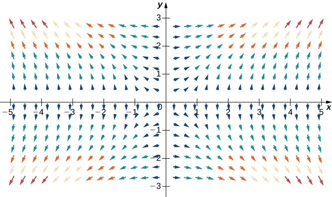
Relationship Between Gradient Fields and Level Curves
Figure 3 shows the level curves of function [latex]f(x,y) = x^2y^2[/latex] overlaid on its gradient vector field. Notice two important patterns:
- The gradient vectors are perpendicular to the level curves
- The magnitudes of the vectors increase as level curves get closer together
These patterns make sense geometrically. Closely grouped level curves indicate the graph is steep, and the magnitude of the gradient vector gives the largest value of the directional derivative. You can assess the local steepness of a graph by examining the corresponding function’s gradient field.
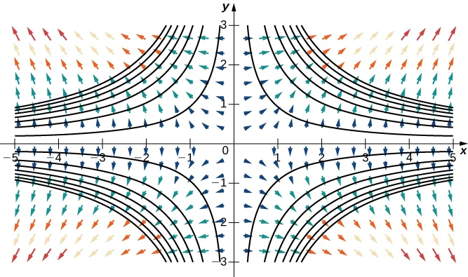
Gradient Direction and Level Curves
The gradient always points in the direction of greatest increase of the function [latex]f[/latex], which is perpendicular to the level curves. This is why:
- Gradient vectors are perpendicular to level curves
- Where the function changes rapidly (closely spaced level curves), gradient vectors are large
- Where the function changes slowly (widely spaced level curves), gradient vectors are small
Potential Functions
A vector field [latex]\mathbf{F}[/latex] is a conservative vector field (or gradient field) if there exists a scalar function [latex]f[/latex] such that [latex]\nabla f = \mathbf{F}[/latex]. In this situation, [latex]f[/latex] is called a potential function for [latex]\mathbf{F}[/latex].
Conservative vector fields arise in many applications, particularly in physics. They are called “conservative” because they model forces in physical systems where energy is conserved. We study conservative vector fields in more detail later in this chapter.
In some physics contexts, a potential function [latex]f[/latex] for [latex]\mathbf{F}[/latex] is defined such that [latex]-\nabla f = \mathbf{F}[/latex] instead of [latex]\nabla f = \mathbf{F}[/latex]. Always check which convention is being used in your specific application.
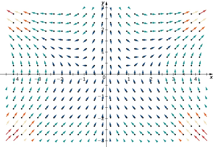
Is [latex]f(x,y,z)=x^2yz-\sin{(xy)}[/latex] a potential function for vector field [latex]{\bf{F}}(x,y,z)=\langle2xyz-y\cos{(xy)},x^2z-x\cos{(xy)},x^2y\rangle[/latex]?
Uniqueness of Potential Functions
If [latex]\mathbf{F}[/latex] is a conservative vector field, is there more than one potential function? If so, how are different potential functions related?
Antiderivatives in Single-Variable Calculus
If [latex]k(x)[/latex] is an integrable function:
- [latex]k[/latex] has infinitely many antiderivatives
- If [latex]F[/latex] and [latex]G[/latex] are both antiderivatives of [latex]k[/latex], then [latex]F(x) = G(x) + C[/latex] for some constant [latex]C[/latex]
The same principle applies to potential functions, since the gradient is like a derivative.
For a conservative vector field [latex]\mathbf{F}[/latex] with potential functions [latex]f[/latex] and [latex]g[/latex], since the gradient is analogous to a derivative, we expect [latex]f(x) = g(x) + C[/latex] for some constant [latex]C[/latex]. The next theorem confirms this.
To state the theorem precisely, we need the domain of the vector field to be connected and open. A domain is connected if you can walk from any point [latex]P_1[/latex] to any other point [latex]P_2[/latex] along a path that stays entirely inside the domain.
uniqueness of potential functions
Let [latex]\mathbf{F}[/latex] be a conservative vector field on an open and connected domain, and let [latex]f[/latex] and [latex]g[/latex] be functions such that [latex]\nabla f = \mathbf{F}[/latex] and [latex]\nabla g = \mathbf{F}[/latex]. Then there is a constant [latex]C[/latex] such that [latex]f = g + C[/latex].
Proof
Since [latex]f[/latex] and [latex]g[/latex] are both potential functions for [latex]\bf{F}[/latex], then [latex]\nabla{(f-g)}=\nabla{f}-\nabla{g}={\bf{F}}-{\bf{F}}=0[/latex]. Let [latex]h=f-g[/latex] then we have [latex]\nabla{h}=0[/latex]. We would like to show that [latex]h[/latex] is a constant function.
Assume [latex]h[/latex] is a function of [latex]x[/latex] and [latex]y[/latex] (the logic of this proof extends to any number of independent variables). Since [latex]\nabla{h}=0[/latex], we have [latex]h_x=0[/latex] and [latex]h_y=0[/latex]. The expression [latex]h_x=0[/latex] implies that [latex]h[/latex] is a constant function with respect to [latex]x[/latex]—that is, [latex]h(x, y)=k_1(y)[/latex] for some function [latex]k_1[/latex]. Similarly, [latex]h_y=0[/latex] implies [latex]h(x, y)=k_2(x)[/latex] for some function [latex]k_2[/latex]. Therefore, function [latex]h[/latex] depends only on [latex]y[/latex] and also depends only on [latex]x[/latex]. Thus, [latex]h(x, y)=C[/latex] for some constant [latex]C[/latex] on the connected domain of [latex]\bf{F}[/latex]. Note that we really do need connectedness at this point; if the domain of [latex]\bf{F}[/latex] came in two separate pieces, then [latex]k[/latex] could be a constant [latex]C_1[/latex] on one piece but could be a different constant [latex]C_2[/latex] on the other piece. Since [latex]f-g=h=C[/latex], we have that [latex]f=g+C[/latex], as desired.
[latex]_\blacksquare[/latex]
The Cross-Partial Property
Conservative vector fields have a special property, called the cross-partial property, that provides a test for whether a given vector field is conservative.
the cross-partial property of conservative vector fields
Let [latex]\mathbf{F}[/latex] be a vector field such that the component functions have continuous second-order mixed-partial derivatives.
In [latex]\mathbb{R}^2[/latex]: If [latex]\mathbf{F}(x,y) = \langle P(x,y), Q(x,y) \rangle[/latex] is conservative, then:
[latex]\dfrac{\partial P}{\partial y} = \dfrac{\partial Q}{\partial x}[/latex]
In [latex]\mathbb{R}^3[/latex]: If [latex]\mathbf{F}(x,y,z) = \langle P(x,y,z), Q(x,y,z), R(x,y,z) \rangle[/latex] is conservative, then:
[latex]\dfrac{\partial P}{\partial y} = \dfrac{\partial Q}{\partial x}, \quad \dfrac{\partial Q}{\partial z} = \dfrac{\partial R}{\partial y}, \quad \text{and} \quad \dfrac{\partial R}{\partial x} = \dfrac{\partial P}{\partial z}[/latex]
Proof
Since [latex]\bf{F}[/latex] is conservative, there is a function [latex]f(x, y)[/latex] such that [latex]\nabla{f}=\bf{F}[/latex]. Therefore, by the definition of the gradient, [latex]f_x=P[/latex] and [latex]f_y=Q[/latex]. By Clairaut’s theorem, [latex]f_{xy}=f_{yx}[/latex], but, [latex]f_{xy}=P_y[/latex] and [latex]f_{yx}=Q_x[/latex], and thus [latex]P_y=Q_x[/latex].
[latex]_\blacksquare[/latex]
Clairaut’s theorem gives a fast proof of the cross-partial property of conservative vector fields in [latex]\mathbb{R}^3[/latex], just as it did for vector fields in [latex]\mathbb{R}^2[/latex].
For a function [latex]f[/latex] with continuous second partial derivatives:
[latex]f_{xy} = f_{yx}[/latex]
This symmetry of mixed partials is the foundation for the cross-partial property of conservative fields.
The ross-partial property of conservative vector fields theorem shows that most vector fields are not conservative. The cross-partial property is difficult to satisfy in general, so most vector fields won’t have equal cross-partials.
The Cross-Partial Property Theorem says:
- If [latex]\mathbf{F}[/latex] is conservative, then [latex]\mathbf{F}[/latex] has the cross-partial property
This does NOT mean:
- If [latex]\mathbf{F}[/latex] has the cross-partial property, then [latex]\mathbf{F}[/latex] is conservative
The theorem can only help you determine that a field is not conservative (by showing the cross-partial property fails). It cannot by itself prove a field is conservative.
For example, vector field [latex]\mathbf{F}(x,y) = \langle x^2y, \frac{x^3}{3} \rangle[/latex] has the cross-partial property, but we cannot use this theorem alone to conclude the field is conservative.