The Main Idea 

A vector field assigns a vector to each point in space, describing phenomena where both magnitude and direction matter at every location. Think of a weather map showing wind velocity—at each point, an arrow indicates wind direction and its length shows speed. Vector fields model gravitational forces, fluid flow, electromagnetic fields, and many other physical systems.

In two dimensions, a vector field [latex]\mathbf{F}[/latex] assigns a two-dimensional vector [latex]\mathbf{F}(x,y)[/latex] to each point latex[/latex] in its domain. In three dimensions, it assigns [latex]\mathbf{F}(x,y,z)[/latex] to each point latex[/latex]. You can think of a vector field as a function whose inputs are points and outputs are vectors.

Representing Vector Fields

A vector field in [latex]\mathbb{R}^2[/latex] can be written in two equivalent forms:

• Component form: [latex]\mathbf{F}(x,y) = \langle P(x,y), Q(x,y) \rangle[/latex]
• Standard unit vector form: [latex]\mathbf{F}(x,y) = P(x,y)\mathbf{i} + Q(x,y)\mathbf{j}[/latex]

The functions [latex]P(x,y)[/latex] and [latex]Q(x,y)[/latex] are the component functions—[latex]P[/latex] gives the horizontal component and [latex]Q[/latex] gives the vertical component. A vector field is continuous if both component functions are continuous.

Physical Interpretation

Vector fields naturally describe physical situations. In a gravitational field, each vector shows the force acting on a unit mass at that point—larger vectors near massive objects indicate stronger gravitational pull. In a velocity field representing water flow, each vector shows the water’s velocity at that location—longer vectors indicate faster flow, and the direction shows which way the water moves.

Visualizing Vector Fields

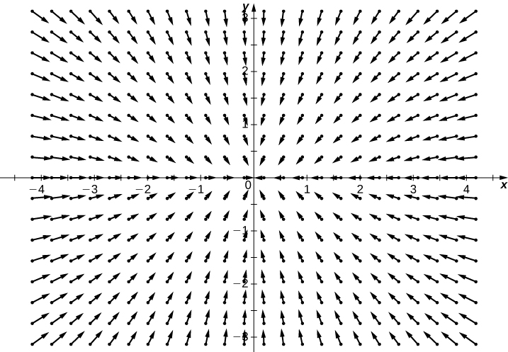
At each point in the domain, draw an arrow representing the vector at that point. The arrow’s direction shows the vector’s direction, and its length represents magnitude. Regions with longer arrows have greater magnitude; regions with shorter arrows have lesser magnitude. The pattern of arrows reveals the overall structure of the field.

The Main Idea 

To visualize a vector field, draw representative vectors at their associated points. For [latex]\mathbf{F}(x,y)[/latex], evaluate the vector at point [latex](x,y)[/latex] and draw it starting from that location. Choose enough points to reveal the pattern without creating clutter—typically grid intersections from each quadrant work well.

Radial Fields

Radial fields have vectors pointing directly toward or away from the origin. All vectors are perpendicular to circles centered at the origin, and magnitude depends only on distance from center. Points on the same circle have equal-magnitude vectors. These model gravitational fields (pointing inward) or energy sources (pointing outward).

Rotational Fields

Rotational fields have vectors tangent to circles around the origin, rotating either clockwise or counterclockwise. Magnitude depends on distance from origin. To verify a field is rotational, check that [latex]\mathbf{F}(a,b) \cdot \langle a,b \rangle = 0[/latex]—the field vector is perpendicular to the radial direction. These model vortices and whirlpools.

Unit Vector Fields

A unit vector field has [latex]||\mathbf{F}(x,y)|| = 1[/latex] everywhere—all vectors have magnitude one. To create a unit vector field from [latex]\mathbf{F}[/latex], normalize by dividing: [latex]\frac{\mathbf{F}}{||\mathbf{F}||}[/latex]. This shows direction without magnitude, useful when only flow pattern matters, not speed.

Vector Fields in [latex]\mathbb{R}^3[/latex]

Three-dimensional fields use three components: [latex]\mathbf{F}(x,y,z) = \langle P(x,y,z), Q(x,y,z), R(x,y,z) \rangle[/latex]. To visualize, first understand behavior in coordinate planes, then see how vectors change moving perpendicular to those planes. Choose representative points from different octants.

The Main Idea 

A gradient field (also called a conservative field) arises when a vector field equals the gradient of some scalar function. These fields model physical systems where energy is conserved, such as gravitational and electrostatic forces. Understanding gradient fields reveals important connections between scalar functions and vector fields.

What is a Gradient Field?

Vector field [latex]\mathbf{F}[/latex] is a gradient field if there exists a scalar function [latex]f[/latex] such that [latex]\nabla f = \mathbf{F}[/latex]. The function [latex]f[/latex] is called a potential function for [latex]\mathbf{F}[/latex]. For two variables, [latex]\nabla f = \langle f_x, f_y \rangle[/latex]. For three variables, [latex]\nabla f = \langle f_x, f_y, f_z \rangle[/latex].

Relationship to Level Curves

Gradient vectors are always perpendicular to level curves of the function. Where level curves are closely spaced (steep regions), gradient vectors have large magnitude. Where level curves are widely spaced (gradual regions), gradient vectors have small magnitude. This makes sense because the gradient points in the direction of greatest increase.

Potential Functions

If [latex]\mathbf{F}[/latex] is conservative with potential functions [latex]f[/latex] and [latex]g[/latex], then [latex]f = g + C[/latex] for some constant [latex]C[/latex]. This parallels how antiderivatives differ by constants in single-variable calculus. Potential functions are unique up to an additive constant.

The Cross-Partial Property

Conservative fields satisfy special equations called the cross-partial property. In [latex]\mathbb{R}^2[/latex], if [latex]\mathbf{F} = \langle P, Q \rangle[/latex] is conservative, then [latex]\frac{\partial P}{\partial y} = \frac{\partial Q}{\partial x}[/latex]. In [latex]\mathbb{R}^3[/latex], three equations must hold: [latex]P_y = Q_x[/latex], [latex]Q_z = R_y[/latex], and [latex]R_x = P_z[/latex]. These come from Clairaut’s theorem: [latex]f_{xy} = f_{yx}[/latex].

Important Limitation

If a field fails the cross-partial property, it’s definitely not conservative. However, satisfying the cross-partial property doesn’t guarantee the field is conservative—it’s necessary but not sufficient. Most vector fields are not conservative since the cross-partial equations are restrictive.