- Apply the circulation form of Green’s theorem
- Apply the flux form of Green’s theorem
- Calculate circulation and flux on general regions
Green’s Theorem
Green’s theorem extends the Fundamental Theorem of Calculus to two dimensions. It has two forms: a circulation form and a flux form, both of which require region [latex]D[/latex] in the double integral to be simply connected. Later, we’ll extend Green’s theorem to regions that are not simply connected.
Green’s theorem relates a line integral around a simply closed plane curve [latex]C[/latex] and a double integral over the region enclosed by [latex]C[/latex]. The theorem is useful because it allows us to translate difficult line integrals into simpler double integrals, or difficult double integrals into simpler line integrals.
Recall that the Fundamental Theorem of Calculus says that:
[latex]\displaystyle\int_a^bF^\prime(x)dx=F(b)-F(a)[/latex].
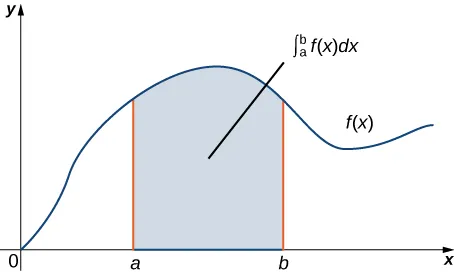
Geometrically, this equation tells us that the integral over the region below the graph of [latex]F^\prime(x)[/latex] and above the line segment [latex][a,b][/latex] depends only on the value of [latex]F[/latex] at the endpoints [latex]a[/latex] and [latex]b[/latex]. Since the numbers [latex]a[/latex] and [latex]b[/latex] form the boundary of line segment [latex][a,b][/latex], we can calculate the integral based on information about the boundary (Figure 1).
The Fundamental Theorem for Line Integrals works the same way:
[latex]\displaystyle\int_C\nabla f\cdot d\mathbf{r}=f(\mathbf{r}(b))-f(\mathbf{r}(a))[/latex].
When we have a potential function (an “antiderivative”), we can calculate the line integral based solely on information about the boundary of curve [latex]C[/latex].
Green’s theorem extends this idea to double integrals. It says we can calculate a double integral over region [latex]D[/latex] based solely on information about the boundary of [latex]D[/latex]. It also says we can calculate a line integral over a simple closed curve [latex]C[/latex] based solely on information about the region that [latex]C[/latex] encloses. Green’s theorem connects a double integral over region [latex]D[/latex] to a line integral around the boundary of [latex]D[/latex].