Limits and Continuity: Learn It 1

Giselle Miller

Limits and Continuity: Learn It 1

Calculate the limit of a function of two variables
Learn how a function of two variables can approach different values at a boundary point, depending on the path of approach
Determine when a function is continuous and check the conditions for continuity
Find limits and check continuity for functions of three or more variables

Limits

We have now examined functions of more than one variable and seen how to graph them. In this section, we see how to take the limit of a function of more than one variable, and what it means for a function of more than one variable to be continuous at a point in its domain. It turns out these concepts have aspects that just don’t occur with functions of one variable.

Limit of a Function of One Variable

Let [latex]f(x)[/latex] be defined for all [latex]x\neq a[/latex] in an open interval containing [latex]a[/latex]. Let [latex]L[/latex] be a real number. Then

[latex]\underset{x\to a}{\text{lim}}f(x)=L[/latex]

if for every [latex]\epsilon>0[/latex], there exists a [latex]\delta>0[/latex], such that if [latex]0<|x-a|<\delta[/latex] for all [latex]x[/latex] in the domain of [latex]f[/latex], then

[latex]|f(x)-L|<\epsilon[/latex].

Before we can adapt this definition to define a limit of a function of two variables, we first need to extend the idea of an open interval in one variable to an open interval in two variables.

[latex]\delta[/latex] disk

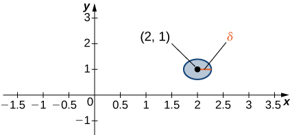
A [latex]\delta[/latex] disk centered at point [latex](a,\ b)[/latex] is an open disk of radius [latex]\delta[/latex] centered at point [latex](a,\ b)[/latex]:

[latex]{(x,y)\in\mathbb{R}^{2},|,(x-a)^{2}+(y-b)^{2}<\delta^{2}}[/latex]

On the xy plane, the point (2, 1) is shown, which is the center of a circle of radius δ. — Figure 1. A [latex]\delta[/latex] disk centered around the point [latex](2,1)[/latex].

The idea of a [latex]\delta[/latex] disk appears in the definition of the limit of a function of two variables. If [latex]\delta[/latex] is small, then all the points [latex](x,\ y)[/latex] in the [latex]\delta[/latex] disk are close to [latex](a,\ b)[/latex]. This is completely analogous to [latex]x[/latex] being close to [latex]a[/latex] in the definition of a limit of a function of one variable. In one dimension, we express this restriction as

[latex]a-\delta

In more than one dimension, we use a [latex]\delta[/latex] disk.

limit of a function of two variables

Let [latex]f[/latex] be a function of two variables. The limit of [latex]f(x,y)[/latex] as [latex](x,\ y)[/latex] approaches [latex](a,\ b)[/latex] is [latex]L[/latex], written:

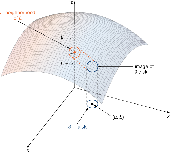
[latex]\underset{(x,y)\to(a,b)}{\text{lim}}f(x,y)=L[/latex]

if for each [latex]\epsilon>0[/latex] there exists a [latex]\delta>0[/latex] such that for all points [latex](x,\ y)[/latex] in a [latex]\delta[/latex] disk around [latex](a,\ b)[/latex], except possibly for [latex](a,\ b)[/latex] itself, we have:

[latex]|f(x,y)-L|<\epsilon[/latex]

In symbols:

For any [latex]\varepsilon>0[/latex], there exists [latex]\delta>0[/latex] such that [latex]|f(x,y)-L|<\varepsilon[/latex] whenever [latex]0<\sqrt{(x-a)^{2}+(y-b)^{2}}<\delta[/latex]

In xyz space, a function is drawn with point L. This point L is the center of a circle of radius ॉ, with points L ± ॉ marked. On the xy plane, there is a point (a, b) drawn with a circle of radius δ around it. This is denoted the δ-disk. There are dashed lines up from the δ-disk to make a disk on the function, which is called the image of delta disk. Then there are dashed lines from this disk to the circle around the point L, which is called the ॉ-neighborhood of L. — Figure 2. The limit of a function involving two variables requires that [latex]f(x,y)[/latex] be within [latex]\varepsilon[/latex] of [latex]L[/latex] whenever [latex](x,y)[/latex] is within [latex]\delta[/latex] of [latex](a,b)[/latex]. The smaller the value of [latex]\varepsilon[/latex], the smaller the value of [latex]\delta[/latex].

Proving that a limit exists using the definition of a limit of a function of two variables can be challenging. Instead, we use the following theorem, which gives us shortcuts to finding limits. The formulas in this theorem are extensions of the formulas in the limit laws theorem for single-variable functions.

limit laws for functions of two variables theorem

Let [latex]\underset{(x,y)\to(a,b)}{\text{lim}}f(x,y)=L[/latex] and [latex]\underset{(x,y)\to(a,b)}{\text{lim}}g(x,y)=M[/latex], and let [latex]c[/latex] be a constant. Then:

Constant Law:

[latex]\displaystyle\lim_{(x,\ y)\to(a,\ b)}c=c[/latex]

Identity Law:

[latex]\begin{array}{ccc}\hfill {\displaystyle\lim_{(x,\ y)\to(a,\ b)}x} & =\hfill & {a} \hfill \\ \hfill {\displaystyle\lim_{(x,\ y)\to(a,\ b)}y} & =\hfill & {b} \end{array}[/latex]

Sum Law:

[latex]\displaystyle\lim_{(x,\ y)\to(a,\ b)}(f\,(x,\ y)+g\,(x,\ y))=L+M[/latex]

Difference Law:

[latex]\displaystyle\lim_{(x,\ y)\to(a,\ b)}(f\,(x,\ y)-(g\,(x,\ y))=L-M[/latex]

Constant Multiple Law:

[latex]\displaystyle\lim_{(x,\ y)\to(a,\ b)}(cf\,(x,\ y))=cL[/latex]

Product Law:

[latex]\displaystyle\lim_{(x,\ y)\to(a,\ b)}(f\,(x,\ y)\,g\,(x,\ y))=LM[/latex]

Quotient Law:

[latex]\displaystyle\lim_{(x,\ y)\to(a,\ b)}\frac{f\,(x,\ y)}{g\,(x,\ y)}=\frac{L}{M}[/latex]

for [latex]M\neq{0}[/latex]

Power Law:

[latex]\displaystyle\lim_{(x,\ y)\to(a,\ b)}(f\,(x,\ y))^{n}=L^{n}[/latex]

for any positive integer [latex]n[/latex].

Root Law:

[latex]\displaystyle\lim_{(x,\ y)\to(a,\ b)}\sqrt[n]{f\,(x,\ y)}=\sqrt[n]{L}[/latex]

for all [latex]L[/latex] if [latex]n[/latex] is odd and positive, and for [latex]L\,\geq\,0[/latex] if [latex]n[/latex] is even and positive.

The proofs of these properties are similar to those for the limits of functions of one variable. We can apply these laws to finding limits of various functions.

Find each of the following limits:

[latex]\displaystyle\lim_{(x,\ y)\to(2,\ -1)}(x^{2}-2xy+3y^{2}-4x+3y-6)[/latex]
[latex]\displaystyle\lim_{(x,\ y)\to(2,\ -1)}\frac{2x+3y}{4x-3y}[/latex]

First use the sum and difference laws to separate the terms:

[latex]\hspace{5cm}\displaystyle\lim_{(x,\ y)\to(2,\ -1)}(x^{2}-2xy+3y^{2}-4x+3y-6)[/latex]

[latex]\hspace{5cm}=\bigg(\displaystyle\lim_{(x,\ y)\to(2,\ -1)}x^{2}\bigg)-\bigg(\displaystyle\lim_{(x,\ y)\to(2,\ -1)}2xy\bigg) +\bigg(\displaystyle\lim_{(x,\ y)\to(2,\ -1)}3y^{2}\bigg)-\bigg(\displaystyle\lim_{(x,\ y)\to(2,\ -1)}4x\bigg) \\ \hspace{5cm}+\bigg(\displaystyle\lim_{(x,\ y)\to(2,\ -1)}3y\bigg)-\bigg(\displaystyle\lim_{(x,\ y)\to(2,\ -1)}6\bigg).[/latex]

Next, use the constant multiple law on the second, third, fourth, and fifth limits:

[latex]\hspace{5cm}=\bigg(\displaystyle\lim_{(x,\ y)\to(2,\ -1)}x^{2}\bigg)-2\bigg(\displaystyle\lim_{(x,\ y)\to(2,\ -1)}xy\bigg)+3\bigg(\displaystyle\lim_{(x,\ y)\to(2,\ -1)}y^{2}\bigg)-4\bigg(\displaystyle\lim_{(x,\ y)\to(2,\ -1)}x\bigg) \\ \hspace{5cm} +3\bigg(\displaystyle\lim_{(x,\ y)\to(2,\ -1)}y\bigg)-\bigg(\displaystyle\lim_{(x,\ y)\to(2,\ -1)}6\bigg).[/latex]

Now, use the power law on the first and third limits, and the product law on the second limit:

[latex]\hspace{5cm} =\bigg(\displaystyle\lim_{(x,\ y)\to(2,\ -1)}x\bigg)^{2}-2\bigg(\displaystyle\lim_{(x,\ y)\to(2,\ -1)}xy\bigg)+3\bigg(\displaystyle\lim_{(x,\ y)\to(2,\ -1)}y\bigg)^{2} \\ \hspace{5cm} -4\bigg(\displaystyle\lim_{(x,\ y)\to(2,\ -1)}x\bigg)+3\bigg(\displaystyle\lim_{(x,\ y)\to(2,\ -1)}y\bigg)-\bigg(\displaystyle\lim_{(x,\ y)\to(2,\ -1)}6\bigg).[/latex]

Last, use the identity laws on the first six limits and the constant law on the last limit:

[latex]\begin{array}{ccc}\hfill{\displaystyle\lim_{(x,\ y)\to(2,\ -1)}(x^{2}-2xy+3y^{2}-4x+3y-6)}& =\hfill & {(2)^{2}-2(2)(-1)+3(-1)^{2}-4(2)+3(-1)-6} \hfill \\ \hfill & =\hfill & {-6} \hfill \\ \hfill \end{array}[/latex]

Before applying the quotient law, we need to verify that the limit of the denominator is nonzero. Using the difference law, constant multiple law, and identity law,
[latex]\begin{array}{ccc}\hfill {\displaystyle\lim_{(x,\ y)\to(2,\ -1)}(4x-3y)} & =\hfill & {\displaystyle\lim_{(x,\ y)\to(2,\ -1)}4x-\displaystyle\lim_{(x,\ y)\to(2,\ -1)}3y}\hfill \\ \hfill & =\hfill & {4\big(\displaystyle\lim_{(x,\ y)\to(2,\ -1)}x\big)-3\big(\displaystyle\lim_{(x,\ y)\to(2,\ -1)}y\big)} \hfill \\ \hfill & =\hfill & {4(2)-3(-1)=11.}\hfill \\ \hfill \end{array}[/latex]

Since the limit of the denominator is nonzero, the quotient law applies. We now calculate the limit of the numerator using the difference law, constant multiple law, and identity law:

[latex]\begin{array}{ccc}\hfill {\displaystyle\lim_{(x,\ y)\to(2,\ -1)}(2x+3y)} & =\hfill & {\displaystyle\lim_{(x,\ y)\to(2,\ -1)}2x+\displaystyle\lim_{(x,\ y)\to(2,\ -1)}3y}\hfill \\ \hfill & =\hfill & {2\big(\displaystyle\lim_{(x,\ y)\to(2,\ -1)}x\big)+3\big(\displaystyle\lim_{(x,\ y)\to(2,\ -1)}y\big)} \hfill \\ \hfill & =\hfill & {2(2)+3(-1)}\hfill \\ \hfill & =\hfill & {1.}\hfill \\ \hfill \end{array}[/latex]

Therefore, according to the quotient law we have

[latex]\displaystyle\lim_{(x,\ y)\to(2,\ -1)}\frac{2x+3y}{4x-3y}=\frac{\displaystyle\lim_{(x,\ y)\to(2,\ -1)}(2x+3y)}{\displaystyle\lim_{(x,\ y)\to(2,\ -1)}(4x-3y)}=\frac{1}{11}.[/latex]

Since we are taking the limit of a function of two variables, the point [latex](a,\ b)[/latex] is in [latex]\mathbb{R}^{2}[/latex], and it is possible to approach this point from an infinite number of directions. Sometimes when calculating a limit, the answer varies depending on the path taken toward [latex](a,\ b)[/latex]. If this is the case, then the limit fails to exist. In other words, the limit must be unique, regardless of path taken

Show that neither of the following limits exist:

[latex]\displaystyle\lim_{(x,\ y)\to(0,\ 0)}\frac{2xy}{3x^{2}+y^{2}}[/latex]
[latex]\displaystyle\lim_{(x,\ y)\to(0,\ 0)}\frac{4xy^{2}}{x^{2}+3y^{4}}[/latex]

The domain of the function [latex]f\,(x,\ y)=\frac{2xy}{3x^{2}+y^{2}}[/latex] consists of all points in the [latex]xy[/latex]-plane except for the point [latex](0,\ 0)[/latex] (Figure 3). To show that the limit does not exist as [latex](x,\ y)[/latex] approaches [latex](0,\ 0)[/latex], we note that it is impossible to satisfy the definition of a limit of a function of two variables because of the fact that the function takes different values along different lines passing through point [latex](0,\ 0)[/latex]. First, consider the line [latex]y=0[/latex] in the [latex]xy[/latex]-plane. Substituting [latex]y=0[/latex] into [latex]f\,(x,\ y)[/latex] gives
[latex]\large{f\,(x,\ 0)=\frac{2x(0)}{3x^{2}+0^{2}}=0}[/latex]

For any value of [latex]x[/latex]. Therefore the value of [latex]f[/latex] remains constant for any point on the [latex]x[/latex]-axis, and as [latex]y[/latex] approaches zero, the function remains fixed at zero. Next, consider the line [latex]y=x[/latex]. Substituting [latex]y=x[/latex] into [latex]f\,(x,\ y)[/latex] gives

[latex]\large{f\,(x,\ x)=\frac{2x(x)}{3x^{2}+x^{2}}=\frac{2x^{2}}{4x^{2}}=\frac{1}{2}}.[/latex]

This is true for any point on the line [latex]y=x[/latex]. If we let [latex]x[/latex] approach zero while staying on this line, the value of the function remains fixed at [latex]\frac{1}{2}[/latex], regardless of how small [latex]x[/latex] is. Choose a value for [latex]\epsilon[/latex] that is less than [latex]1/2-[/latex]say, [latex]1/4[/latex]. Then, no matter how small a [latex]\delta[/latex] disk we draw around [latex](0,\ 0)[/latex], the values of [latex]f\,(x,\ y)[/latex] for points inside that [latex]\delta[/latex] disk will include both [latex]0[/latex] and [latex]\frac{1}{2}.[/latex] Therefore, the definition of limit at a point is never satisfied and the limit fails to exist.

Figure 3. Graph of the function [latex]\small{f(x,y)=(2xy)/(3x^{2}+y^{2})}[/latex]. Along the line [latex]\small{y=0}[/latex], the function is equal to zero; along the line [latex]\small{y=x}[/latex], the function is equal to [latex]\small{\frac{1}{2}}[/latex].
In a similar fashion to 1., we can approach the origin along any straight line passing through the origin. If we try the [latex]x[/latex]-axis (i.e., [latex]y=0[/latex]), then the function remains fixed at zero. The same is true for the [latex]y[/latex]-axis. Suppose we approach the origin along a straight line of slope [latex]k[/latex] The equation of this line is [latex]y=kx[/latex]. Then the limit becomes
[latex]\begin{array}{ccc}\hfill {\displaystyle\lim_{(x,\ y)\to(0,\ 0)}\frac{4xy^{2}}{x^{2}+3y^{4}}} & =\hfill & {\displaystyle\lim_{(x,\ y)\to(0,\ 0)}\frac{4x(kx)^{2}}{x^{2}+3(kx)^{4}}}\hfill \\ \hfill & =\hfill & {\displaystyle\lim_{(x,\ y)\to(0,\ 0)}\frac{4k^{2}x^{3}}{x^{2}+3k^{4}x^{4}}} \hfill \\ \hfill & =\hfill & {\displaystyle\lim_{(x,\ y)\to(0,\ 0)}\frac{4k^{2}x}{1+3k^{4}x^{2}}}\hfill \\ \hfill & =\hfill & {\frac{\displaystyle\lim_{(x,\ y)\to(0,\ 0)}4k^{2}x}{\displaystyle\lim_{(x,\ y)\to(0,\ 0)}(1+3k^{4}x^{2})}}\hfill \\ \hfill & =\hfill & {0}\hfill \\ \hfill \end{array}[/latex]

Regardless of the value of [latex]k[/latex]. It would seem that the limit is equal to zero. What if we chose a curve passing through the origin instead? For example, we can consider the parabola given by the equation [latex]x=y^{2}[/latex]. Substituting [latex]y^{2}[/latex] in place of [latex]x[/latex] in [latex]f\,(x,\ y)[/latex] gives

[latex]\begin{array}{ccc}\hfill {\displaystyle\lim_{(x,\ y)\to(0,\ 0)}\frac{4xy^{2}}{x^{2}+3y^{4}}} & =\hfill & {\displaystyle\lim_{(x,\ y)\to(0,\ 0)}\frac{4(y^{2})y^{2}}{(y^{2})^{2}+3y^{4}}}\hfill \\ \hfill & =\hfill & {\displaystyle\lim_{(x,\ y)\to(0,\ 0)}\frac{4y^{4}}{y^{4}+3y^{4}}} \hfill \\ \hfill & =\hfill & {\displaystyle\lim_{(x,\ y)\to(0,\ 0)}1}\hfill \\ \hfill & =\hfill & {1.}\hfill \\ \hfill \end{array}[/latex]

By the same logic in 1., it is impossible to find a [latex]\delta[/latex] disk around the origin that satisfies the definition of the limit for any value of [latex]\epsilon\,<\,1[/latex]. Therefore, [latex]\displaystyle\lim_{(x,\ y)\to(0,\ 0)}\frac{4xy^{2}}{x^{2}+3y^{4}}[/latex] does not exist.