- Describe how particles move in space using velocity and acceleration vectors
- Explain the tangential and normal components of acceleration
- Use vector-valued functions to describe and analyze planetary motion
Motion Vectors in the Plane and in Space
You now know how to describe curves in the plane and in space, and how to determine their properties like arc length and curvature. These tools come together to describe motion along curves—the main goal of this chapter.
Our starting point is using vector-valued functions to represent the position of an object as a function of time. This approach works for both plane curves and space curves. For example, planetary orbits are elliptical curves that lie in a plane, while a particle traveling along a helix moves through three-dimensional space.
position, velocity, acceleration, and speed
Let [latex]{\bf{r}}(t)[/latex] be a twice-differentiable vector-valued function of the parameter [latex]t[/latex] that represents the position of an object as a function of time.
- Velocity vector: [latex]{\bf{v}}(t)={\bf{r}}'(t)[/latex]
- Acceleration vector: [latex]{\bf{a}}(t)={\bf{v}}'(t)={\bf{r}}''(t)[/latex]
- Speed: [latex]v(t)=\left\Vert{\bf{v}}(t)\right\Vert=\left\Vert{\bf{r}}'(t)\right\Vert=\frac{ds}{dt}[/latex]
Since [latex]{\bf{r}}(t)[/latex] can describe motion in either two or three dimensions, these vector-valued functions can have either two or three components. In two dimensions, we write [latex]{\bf{r}}(t)=x(t){\bf{i}}+y(t){\bf{j}}[/latex], and in three dimensions [latex]{\bf{r}}(t)=x(t){\bf{i}}+y(t){\bf{j}}+z(t){\bf{k}}[/latex]. The table below shows how velocity, acceleration, and speed are expressed in each case.
| Quantity | Two Dimensions | Three Dimensions |
|---|---|---|
| Position | [latex]{\bf{r}}(t)=x(t){\bf{i}}+y(t){\bf{j}}[/latex] | [latex]{\bf{r}}(t)=x(t){\bf{i}}+y(t){\bf{j}}+z(t){\bf{k}}[/latex] |
| Velocity | [latex]{\bf{v}}(t)=x'(t){\bf{i}}+y'(t){\bf{j}}[/latex] | [latex]{\bf{v}}(t)=x'(t){\bf{i}}+y'(t){\bf{j}}+z'(t){\bf{k}}[/latex] |
| Acceleration | [latex]{\bf{a}}(t)=x''(t){\bf{i}}+y''(t){\bf{j}}[/latex] | [latex]{\bf{a}}(t)=x''(t){\bf{i}}+y''(t){\bf{j}}+z''(t){\bf{k}}[/latex] |
| Speed | [latex]v(t)=\sqrt{(x'(t))^{2}+(y'(t))^{2}}[/latex] | [latex]v(t)=\sqrt{(x'(t))^{2}+(y'(t))^{2}+(z'(t))^{2}}[/latex] |
- Find the velocity, acceleration, and speed as functions of time.
- Sketch the curve along with the velocity vector at time [latex]t=1[/latex].

Understanding Velocity and Acceleration Vectors
Imagine driving along a curvy road. If you don’t turn the steering wheel, you continue in a straight line and run off the road. The speed and direction at which you leave the road give a vector representing your velocity (Figure 2).
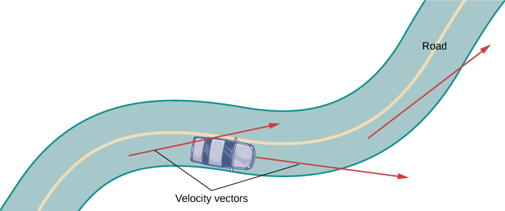
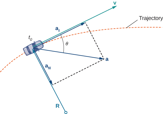
The fact that you must turn the steering wheel to stay on the road shows that your velocity is always changing—even if your speed stays constant—because your direction constantly changes. As you turn right, your acceleration vector points right. As you turn left, your acceleration vector points left. Your velocity and acceleration vectors are constantly changing, regardless of whether your speed varies (Figure 3).
Key Insight About Velocity and Acceleration
- The velocity vector is always tangent to the path of motion
- The acceleration vector points toward the direction the object is turning
- Speed can remain constant even while velocity changes, because velocity depends on both speed and direction