Using the Divergence Theorem

The divergence theorem translates between the flux integral of closed surface [latex]S[/latex] and a triple integral over the solid enclosed by [latex]S[/latex]. Therefore, the theorem allows us to compute flux integrals or triple integrals that would ordinarily be difficult to compute by translating the flux integral into a triple integral and vice versa.

Calculate the surface integral [latex]\displaystyle\iint_{S}{\bf{F}}\cdot d{\bf{S}}[/latex], where [latex]S[/latex] is cylinder [latex]x^2+y^2=1[/latex], [latex]0\leq z\leq2[/latex], including the circular top and bottom, and [latex]{\bf{F}}=\left\langle\frac{x^3}{3}+yz,\frac{y^3}3-\sin(xz),z-x-y\right\rangle[/latex].

Show Solution

We could calculate this integral without the divergence theorem, but the calculation is not straightforward because we would have to break the flux integral into three separate integrals: one for the top of the cylinder, one for the bottom, and one for the side. Furthermore, each integral would require parameterizing the corresponding surface, calculating tangent vectors and their cross product, and using the equation to calculate scalar surface integrals.

By contrast, the divergence theorem allows us to calculate the single triple integral [latex]\displaystyle\iiint_E\text{div }{\bf{F}}dV[/latex], where [latex]E[/latex] is the solid enclosed by the cylinder. Using the divergence theorem and converting to cylindrical coordinates, we have

[latex]\begin{aligned} \displaystyle\iint_S{\bf{F}}\cdot d{\bf{S}}&=\displaystyle\iiint_E\text{div }{\bf{F}}dV \\ &=\displaystyle\iiint_E(x^2+y^2+1)dV \\ &=\displaystyle\int_0^{2\pi}\displaystyle\int_0^1\displaystyle\int_0^2(r^2+1)r \ dzdrd\theta \\ &=\frac32\displaystyle\int_0^{2\pi}d\theta=3\pi \end{aligned}[/latex].

Let [latex]{\bf{v}}=\left\langle-\frac{y}z,\frac{x}z,0\right\rangle[/latex] be the velocity field of a fluid. Let [latex]C[/latex] be the solid cube given by [latex]1\leq x \leq4[/latex], [latex]2\leq y\leq5[/latex], [latex]1\leq z\leq4[/latex], and let [latex]S[/latex] be the boundary of this cube (see the following figure). Find the flow rate of the fluid across [latex]S[/latex].

Show Solution

The flow rate of the fluid across [latex]S[/latex] is [latex]\displaystyle\iint_s{\bf{v}}\cdot d{\bf{S}}[/latex]. Before calculating this flux integral, let’s discuss what the value of the integral should be. Based on Figure 2, we see that if we place this cube in the fluid (as long as the cube doesn’t encompass the origin), then the rate of fluid entering the cube is the same as the rate of fluid exiting the cube. The field is rotational in nature and, for a given circle parallel to the [latex]xy[/latex]-plane that has a center on the [latex]z[/latex]-axis, the vectors along that circle are all the same magnitude. That is how we can see that the flow rate is the same entering and exiting the cube. The flow into the cube cancels with the flow out of the cube, and therefore the flow rate of the fluid across the cube should be zero.

To verify this intuition, we need to calculate the flux integral. Calculating the flux integral directly requires breaking the flux integral into six separate flux integrals, one for each face of the cube. We also need to find tangent vectors, compute their cross product, and use the equation to calculate scalar surface integrals. However, using the divergence theorem makes this calculation go much more quickly:

[latex]\begin{aligned} \displaystyle\iint_s{\bf{v}}\cdot d{\bf{S}}&=\displaystyle\iiint_C\text{div }({\bf{v}})dV \\ &=\displaystyle\iiint_C0 \ dV=0 \end{aligned}[/latex].

Therefore the flux is zero, as expected.

A Special Case: Zero Divergence

The example above illustrates a remarkable consequence of the divergence theorem. Let [latex]S[/latex] be a piecewise, smooth closed surface and let [latex]\mathbf{F}[/latex] be a vector field defined on an open region containing the surface enclosed by [latex]S[/latex].

If [latex]\mathbf{F}[/latex] has the form [latex]\mathbf{F} = \langle f(y,z), g(x,z), h(x,y) \rangle[/latex], then the divergence of [latex]\mathbf{F}[/latex] is zero. By the divergence theorem, the flux of [latex]\mathbf{F}[/latex] across [latex]S[/latex] is also zero. This makes certain flux integrals incredibly easy to calculate.

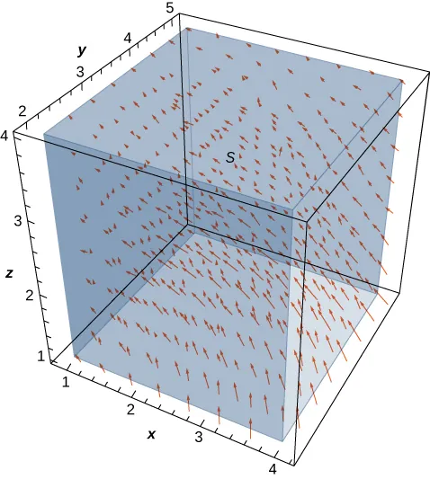
For example, suppose we wanted to calculate the flux integral [latex]\iint_S \mathbf{F} \cdot d\mathbf{S}[/latex] where [latex]S[/latex] is a cube and:

[latex]{\bf{F}}=\langle\sin(y)e^{yz},x^2z^2,\cos(xy)e^{\sin x}\rangle[/latex].

Calculating the flux integral directly would be difficult, if not impossible, using techniques we studied previously. At the very least, we would have to break the flux integral into six integrals, one for each face of the cube. But, because the divergence of this field is zero, the divergence theorem immediately shows that the flux integral is zero.

Quick Check for Zero Flux

If a vector field has the form [latex]\mathbf{F} = \langle f(y,z), g(x,z), h(x,y) \rangle[/latex] (where each component depends only on the two variables shown), then:

• [latex]\text{div } \mathbf{F} = 0[/latex]
• The flux across any closed surface is automatically zero

This can save significant computation time!

Justifying the Physical Interpretation

We can now use the divergence theorem to justify the physical interpretation of divergence that we discussed earlier. Recall that if [latex]\mathbf{F}[/latex] is a continuous three-dimensional vector field and [latex]P[/latex] is a point in the domain of [latex]\mathbf{F}[/latex], then the divergence of [latex]\mathbf{F}[/latex] at [latex]P[/latex] is a measure of the “outflowing-ness” of [latex]\mathbf{F}[/latex] at [latex]P[/latex].

If [latex]\mathbf{F}[/latex] represents the velocity field of a fluid, then the divergence of [latex]\mathbf{F}[/latex] at [latex]P[/latex] is a measure of the net flow rate out of point [latex]P[/latex] (the flow of fluid out of [latex]P[/latex] less the flow of fluid in to [latex]P[/latex]).

To see how the divergence theorem justifies this interpretation, let [latex]B_r[/latex] be a ball of very small radius [latex]r[/latex] with center [latex]P[/latex], and assume that [latex]B_r[/latex] is in the domain of [latex]\mathbf{F}[/latex]. Furthermore, assume that [latex]B_r[/latex] has a positive, outward orientation.

Since the radius of [latex]B_r[/latex] is small and [latex]\mathbf{F}[/latex] is continuous, the divergence of [latex]\mathbf{F}[/latex] is approximately constant on [latex]B_r[/latex]. That is, if [latex]P'[/latex] is any point in [latex]B_r[/latex], then [latex]\text{div } \mathbf{F}(P) \approx \text{div } \mathbf{F}(P')[/latex].

Let [latex]S_r[/latex] denote the boundary sphere of [latex]B_r[/latex]. We can approximate the flux across [latex]S_r[/latex] using the divergence theorem as follows:

[latex]\begin{aligned} \displaystyle\iint_S{\bf{F}}\cdot d{\bf{S}}&=\displaystyle\iiint_{B_r}\text{div }{\bf{F}}dV \\ &\approx\displaystyle\iiint_{B_r}\text{div }{\bf{F}}(P)dV \\ &=\text{div }{\bf{F}}(P)V(B_r) \end{aligned}[/latex].

As we shrink the radius [latex]r[/latex] to zero via a limit, the quantity [latex]\text{div }{\bf{F}}(P)V(B_r)[/latex] gets arbitrarily close to the flux. Therefore:

[latex]\large{\text{div }{\bf{F}}(P)=\displaystyle\lim_{r\to0}\frac{1}{V(B_r)}\displaystyle\iint_{S_r}{\bf{F}}\cdot d{\bf{S}}}[/latex]

and we can consider the divergence at [latex]P[/latex] as measuring the net rate of outward flux per unit volume at [latex]P[/latex]. Since “outflowing-ness” is an informal term for the net rate of outward flux per unit volume, we have justified the physical interpretation of divergence we discussed earlier, and we have used the divergence theorem to give this justification.