Flux and Circulation

We close this section by discussing two key concepts related to line integrals: flux across a plane curve and circulation along a plane curve. Flux is used to calculate fluid flow across a curve, and circulation is important for characterizing conservative gradient fields. Both concepts are used heavily throughout the rest of this course and are especially important for Green’s theorem, Stokes’ theorem, and the divergence theorem.

Understanding Flux

Let [latex]C[/latex] be a plane curve and let [latex]{\textbf{F}}[/latex] be a vector field in the plane. Imagine [latex]C[/latex] is a membrane across which fluid flows, but [latex]C[/latex] does not impede the flow of the fluid. In other words, [latex]C[/latex] is an idealized membrane invisible to the fluid. Suppose [latex]{\textbf{F}}[/latex] represents the velocity field of the fluid. How could we quantify the rate at which the fluid is crossing [latex]C[/latex]?

Recall that the line integral of [latex]{\textbf{F}}[/latex] along [latex]C[/latex] is [latex]\displaystyle\int_C{\textbf{F}}\cdot{\textbf{T}} ds[/latex]—the dot product of the vector field with the unit tangential vector with respect to arc length. If we replace the unit tangential vector with unit normal vector [latex]{\textbf{N}}(t)[/latex] and instead compute integral [latex]\displaystyle\int_C{\textbf{F}}\cdot{\textbf{N}} ds[/latex], we determine the flux across [latex]C[/latex].

The definition of integral [latex]\displaystyle\int_C{\textbf{F}}\cdot{\textbf{N}} ds[/latex] is the same as integral [latex]\displaystyle\int_C{\textbf{F}}\cdot{\textbf{T}} ds[/latex], except the [latex]{\textbf{T}}[/latex] in the Riemann sum is replaced with [latex]{\textbf{N}}[/latex]. Therefore, the flux across [latex]C[/latex] is defined as:

[latex]\displaystyle\int_c{\bf{F}}\cdot{\bf{N}} \ ds=\displaystyle\lim_{n\to\infty}\displaystyle\sum_{i=1}^n{\bf{F}}(P_i^*)\cdot{\bf{N}}(P_i^*)\Delta{s_i}[/latex],

where [latex]P_i^*[/latex] and [latex]\Delta s[/latex] are defined as they were for integral [latex]\displaystyle\int_C{\textbf{F}}\cdot{\textbf{T}} ds[/latex]. A flux integral is perpendicular to a vector line integral, because [latex]{\textbf{N}}[/latex] and [latex]{\textbf{T}}[/latex] are perpendicular vectors.

If [latex]{\textbf{F}}[/latex] is a velocity field of a fluid and [latex]C[/latex] is a curve that represents a membrane, then the flux of [latex]{\textbf{F}}[/latex] across [latex]C[/latex] is the quantity of fluid flowing across [latex]C[/latex] per unit time, or the rate of flow.

More formally, let [latex]C[/latex] be a plane curve parameterized by [latex]{\textbf{r}}(t)=\langle x(t),y(t)\rangle[/latex], [latex]a\leq t\leq b[/latex]. Let [latex]{\textbf{n}}(t)=\langle y'(t),-x'(t)\rangle[/latex] be the vector that is normal to [latex]C[/latex] at the endpoint of [latex]{\textbf{r}}(t)[/latex] and points to the right as we traverse [latex]C[/latex] in the positive direction (Figure 3). Then [latex]{\textbf{N}}(t)=\frac{{\textbf{n}}(t)}{||{\textbf{n}}(t)||}[/latex] is the unit normal vector to [latex]C[/latex] at the endpoint of [latex]{\textbf{r}}(t)[/latex] that points to the right as we traverse [latex]C[/latex].

flux across a curve

The flux of [latex]{\textbf{F}}[/latex] across [latex]C[/latex] is line integral:

[latex]\displaystyle\int_C{\textbf{F}}\cdot\frac{{\textbf{n}}(t)}{||{\textbf{n}}(t)||}ds[/latex]

We now give a formula for calculating the flux across a curve. This formula is analogous to the formula used to calculate a vector line integral.

calculating flux across a curve

Let [latex]{\bf{F}}[/latex] be a vector field and let [latex]C[/latex] be a smooth curve with parameterization [latex]{\bf{r}}(t)=\langle{x}(t),y(t)\rangle[/latex], [latex]a\leq{t}\leq{b}[/latex]. Let [latex]{\bf{n}}(t)=\langle{y}^\prime(t),-x^\prime(t)\rangle[/latex]. The flux of [latex]{\bf{F}}[/latex] across [latex]C[/latex] is:

[latex]\displaystyle\int_C{\bf{F}}\cdot{\bf{N}}ds=\displaystyle\int_a^b{\bf{F}}({\bf{r}}(t))\cdot{\bf{n}}(t)dt[/latex].

Proof

---

The proof of calculating flux across a curve is similar to the proof of the scalar line integral calculation. Before deriving the formula, note that [latex]||{\bf{n}}(t)||=||\langle y'(t),-x'(t)\rangle||=\sqrt{(y^\prime(t))^2+(x^\prime(t))^2}=||{\bf{r}}^\prime(t)||[/latex]. Therefore,

[latex]\begin{aligned} \displaystyle\int_C{\bf{F}}\cdot{\bf{N}}ds&=\displaystyle\int_C{\bf{F}}\cdot\frac{{\bf{n}}}{||{\bf{n}}(t)||}ds \\ &=\displaystyle\int_a^b{\bf{F}}\frac{{\bf{n}}}{||{\bf{n}}(t)||}||{\bf{r}}^\prime(t)||dt \\ &=\displaystyle\int_a^b{\bf{F}}[({\bf{r}}(t))\cdot{\bf{n}}(t)dt \end{aligned}[[/latex].

[latex]_\blacksquare[/latex]

Calculate the flux of [latex]{\bf{F}}=\langle2x,2y\rangle[/latex] across a unit circle oriented counterclockwise (Figure 4).

Show Solution

To compute the flux, we first need a parameterization of the unit circle. We can use the standard parameterization [latex]{\bf{r}}(t)\langle\cos{t},\sin{t}\rangle[/latex], [latex]0\leq{t}\leq2\pi[/latex]. The normal vector to a unit circle is [latex]\langle\cos{t},\sin{t}\rangle[/latex]. Therefore, the flux is

[latex]\begin{aligned} \displaystyle\int_C{\bf{F}}\cdot{\bf{N}}ds&=\displaystyle\int_0^{2\pi}\langle2\cos{t},2\sin{t}\rangle\cdot\langle\cos{t},\sin{t}\rangle \ dt \\ &=\displaystyle\int_0^{2\pi}(2\cos^2{t},2\sin^2{t}) \ dt = 2\displaystyle\int_0^{2\pi}(\cos^2{t},\sin^2{t}) \ dt \\ &=2\displaystyle\int_0^{2\pi} \ dt = 4\pi \end{aligned}[/latex].

Alternative Notation for Flux

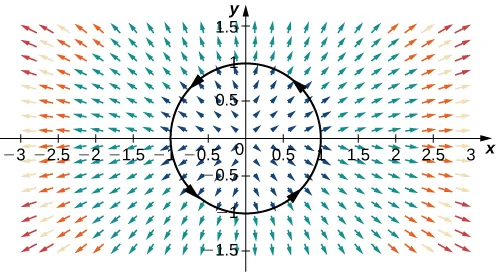
Let [latex]{\textbf{F}}(x,y)=\langle P(x,y),Q(x,y)\rangle[/latex] be a two-dimensional vector field. Recall that integral [latex]\displaystyle\int_C{\textbf{F}}\cdot{\textbf{T}}ds[/latex] is sometimes written as [latex]\displaystyle\int_CP dx+Q dy[/latex].

Analogously, flux [latex]\displaystyle\int_C{\textbf{F}}\cdot{\textbf{N}}ds[/latex] is sometimes written in the notation [latex]\displaystyle\int_C-Q dx+P dy[/latex], because the unit normal vector [latex]{\textbf{N}}[/latex] is perpendicular to the unit tangent [latex]{\textbf{T}}[/latex]. Rotating the vector [latex]d{\textbf{r}}=\langle dx,dy\rangle[/latex] by [latex]90°[/latex] results in vector [latex]\langle dy,-dx\rangle[/latex].

Understanding Circulation

The line integral of vector field [latex]{\textbf{F}}[/latex] along an oriented closed curve is called the circulation of [latex]{\textbf{F}}[/latex] along [latex]C[/latex]. Circulation line integrals have their own notation:

[latex]\displaystyle\oint_C{\textbf{F}}\cdot{\textbf{T}}ds[/latex].

The circle on the integral symbol denotes that [latex]C[/latex] is “circular” in that it has no endpoints.

To see where the term circulation comes from and what it measures, let [latex]{\textbf{v}}[/latex] represent the velocity field of a fluid and let [latex]C[/latex] be an oriented closed curve. At a particular point [latex]P[/latex], the closer the direction of [latex]{\textbf{v}}(P)[/latex] is to the direction of [latex]{\textbf{T}}(P)[/latex], the larger the value of the dot product [latex]{\textbf{v}}(P)\cdot{\textbf{T}}(P)[/latex].

The maximum value of [latex]{\textbf{v}}(P)\cdot{\textbf{T}}(P)[/latex] occurs when the two vectors point in the exact same direction. The minimum value occurs when the two vectors point in opposite directions. Thus, the value of the circulation [latex]\displaystyle\oint_C{\textbf{v}}\cdot{\textbf{T}}ds[/latex] measures the tendency of the fluid to move in the direction of [latex]C[/latex].

Let [latex]{\textbf{F}}=\langle -y,x\rangle[/latex] and let [latex]C[/latex] represent the unit circle oriented counterclockwise. Calculate the circulation of [latex]{\textbf{F}}[/latex] along [latex]C[/latex].

We use the standard parameterization of the unit circle: [latex]{\bf{r}}(t)=\langle\cos{t},\sin{t}\rangle[/latex], [latex]0\leq{t}\leq2\pi[/latex]. Then, [latex]{\bf{F}}({\bf{r}}(t))=\langle-\sin{t},\cos{t}\rangle[/latex] and [latex]{\bf{r}}'(t)=\langle-\sin{t},\cos{t}\rangle[/latex]. Therefore, the circulation of [latex]\bf{F}[/latex] along [latex]C[/latex] is

[latex]\begin{aligned} \displaystyle\oint_C{\bf{F}}\cdot{\bf{T}}ds&=\displaystyle\int_0^{2\pi}\langle-\sin{t},\cos{t}\rangle\cdot\langle-\sin{t},\cos{t}\rangle \ dt \\ &=\displaystyle\int_0^{2\pi}(\sin^2{t}+\cos^2{t}) \ dt \\ &=\displaystyle\int_0^{2\pi} \ dt = 2\pi \end{aligned}[/latex].

Notice that the circulation is positive. The reason for this is that the orientation of [latex]C[/latex] “flows” with the direction of [latex]\bf{F}[/latex]. At any point along the circle, the tangent vector and the vector from [latex]\bf{F}[/latex] form an angle of less than 90°, and therefore the corresponding dot product is positive.