Change of Variables: Learn It 4

Giselle Miller

Change of Variables: Learn It 4

Change of Variables for Triple Integrals

Changing variables in triple integrals works exactly the same way as for double integrals. Cylindrical and spherical coordinate substitutions are special cases of this general method.

Suppose [latex]G[/latex] is a region in [latex]uvw[/latex]-space that maps to region [latex]D[/latex] in [latex]xyz[/latex]-space (Figure 6) by a one-to-one [latex]C^1[/latex] transformation [latex]T(u,v,w) = (x,y,z)[/latex] where:

[latex]x = g(u,v,w)[/latex]
[latex]y = h(u,v,w)[/latex]
[latex]z = k(u,v,w)[/latex]

On the left-hand side of this figure, there is a region G in u v w space. Then there is an arrow from this graph to the right-hand side of the figure marked with x = g(u, v, w), y = h(u, v, w), and z = k(u, v, w). On the right-hand side of this figure there is a region D in xyz space. — Figure 6. A region [latex]G[/latex] in [latex]uvw[/latex]-space mapped to a region [latex]D[/latex] in [latex]xyz[/latex]-space.

Any function [latex]F(x,y,z)[/latex] defined on [latex]D[/latex] can be expressed as a function [latex]H(u,v,w)[/latex] defined on [latex]G[/latex]:

[latex]F(x,y,z)=F(g(u,v,w), \ h(u,v,w) \ k(u,v,w))= \ H(u,v,w)[/latex].

Two-Dimensional Jacobian

For a transformation [latex]T(u,v) = (x,y)[/latex], the Jacobian is the [latex]2 \times 2[/latex] determinant:

[latex]J(u,v) = \begin{vmatrix} \dfrac{\partial x}{\partial u} & \dfrac{\partial y}{\partial u} \\ \dfrac{\partial x}{\partial v} & \dfrac{\partial y}{\partial v} \end{vmatrix}[/latex]

The three-dimensional case extends this to a [latex]3 \times 3[/latex] determinant.

The Jacobian determinant [latex]J(u,v,w)[/latex] in three variables is defined as:

[latex]J(u,v,w) = \begin{vmatrix} \dfrac{\partial x}{\partial u} & \dfrac{\partial y}{\partial u} & \dfrac{\partial z}{\partial u} \\ \dfrac{\partial x}{\partial v} & \dfrac{\partial y}{\partial v} & \dfrac{\partial z}{\partial v} \\ \dfrac{\partial x}{\partial w} & \dfrac{\partial y}{\partial w} & \dfrac{\partial z}{\partial w} \end{vmatrix}[/latex]

This can also be written equivalently as:

[latex]J(u,v,w) = \begin{vmatrix} \dfrac{\partial x}{\partial u} & \dfrac{\partial x}{\partial v} & \dfrac{\partial x}{\partial w} \\ \dfrac{\partial y}{\partial u} & \dfrac{\partial y}{\partial v} & \dfrac{\partial y}{\partial w} \\ \dfrac{\partial z}{\partial u} & \dfrac{\partial z}{\partial v} & \dfrac{\partial z}{\partial w} \end{vmatrix}[/latex]

jacobian determinant in three variables

For transformation [latex]T(u,v,w) = (x,y,z)[/latex]:

[latex]J(u,v,w) = \dfrac{\partial(x,y,z)}{\partial(u,v,w)} = \begin{vmatrix} \dfrac{\partial x}{\partial u} & \dfrac{\partial x}{\partial v} & \dfrac{\partial x}{\partial w} \\ \dfrac{\partial y}{\partial u} & \dfrac{\partial y}{\partial v} & \dfrac{\partial y}{\partial w} \\ \dfrac{\partial z}{\partial u} & \dfrac{\partial z}{\partial v} & \dfrac{\partial z}{\partial w} \end{vmatrix}[/latex]

This determinant measures how the transformation scales volumes.

The Jacobian is commonly denoted simply as [latex]\dfrac{\partial(x,y,z)}{\partial(u,v,w)}[/latex].

Just as with two variables, you can arrange the [latex]3 \times 3[/latex] determinant in two equivalent ways:

By output variables: Rows for [latex]x[/latex], [latex]y[/latex], [latex]z[/latex] derivatives
By input variables: Columns for [latex]u[/latex], [latex]v[/latex], [latex]w[/latex] derivatives

Both give the same result when you compute the determinant.

With the transformation and Jacobian defined, we can state the theorem for changing variables in triple integrals.

change of variables for triple integrals

Let [latex]T(u,v,w) = (x,y,z)[/latex] where [latex]x = g(u,v,w)[/latex], [latex]y = h(u,v,w)[/latex], and [latex]z = k(u,v,w)[/latex] be a one-to-one [latex]C^1[/latex] transformation with a nonzero Jacobian that maps region [latex]G[/latex] in [latex]uvw[/latex]-space into region [latex]D[/latex] in [latex]xyz[/latex]-space. If [latex]F[/latex] is continuous on [latex]D[/latex], then:

[latex]\hspace{3cm}\begin{align} \underset{R}{\displaystyle\iiint}F(x,y,z)dV&=\underset{G}{\displaystyle\iiint}F(g(u,v,w), \ h(u,v,w), \ k(u,v,w))\Bigg|\frac{\partial(x,y,z)}{\partial(u,v,w)}\Bigg|du \ dv \ dw \\ &=\underset{G}{\displaystyle\iiint}H(u,v,w)|J(u,v,w)|du \ dv \ dw \end{align}[/latex].

In other words, when changing variables from [latex](x,y,z)[/latex] to [latex](u,v,w)[/latex]:

[latex]dV = dx \, dy \, dz = | \dfrac{\partial(x,y,z)}{\partial(u,v,w)} | du \, dv \, dw[/latex]

Cylindrical and Spherical Coordinates

The coordinate systems you’ve already used are special cases of this general theorem:

Cylindrical coordinates: [latex]x = r\cos\theta[/latex], [latex]y = r\sin\theta[/latex], [latex]z = z[/latex]

Jacobian: [latex]J(r,\theta,z) = r[/latex]
Volume element: [latex]dV = r , dr , d\theta , dz[/latex]

Spherical coordinates: [latex]x = \rho\sin\phi\cos\theta[/latex], [latex]y = \rho\sin\phi\sin\theta[/latex], [latex]z = \rho\cos\phi[/latex]

Jacobian: [latex]J(\rho,\phi,\theta) = \rho^2\sin\phi[/latex]
Volume element: [latex]dV = \rho^2\sin\phi , d\rho , d\phi , d\theta[/latex]

We’ll verify these formulas using the change of variables theorem.

Derive the formula in triple integrals for

cylindrical and
spherical coordinates.

For cylindrical coordinates, the transformation is [latex]T(r,\theta,z)=(x,y,z)[/latex] from the Cartesian [latex]r\theta{z}[/latex]–plane to the Cartesian [latex]xyz[/latex]-plane (Figure 7). Here [latex]x=r\cos\theta[/latex], [latex]y=r\sin\theta[/latex], and [latex]z=z[/latex]. The Jacobian for the transformation is

[latex]\hspace{1.5cm}\large{\begin{align}J(r,\theta,z)&=\frac{\partial(x,y,z)}{\partial(r,\theta,z)}=\begin{vmatrix}\frac{\partial{x}}{\partial{r}}&\frac{\partial{x}}{\partial{\theta}}&\frac{\partial{x}}{\partial{z}} \\ \frac{\partial{y}}{\partial{r}}&\frac{\partial{y}}{\partial{\theta}}&\frac{\partial{y}}{\partial{z}} \\ \frac{\partial{z}}{\partial{r}}&\frac{\partial{z}}{\partial{\theta}}&\frac{\partial{z}}{\partial{z}}\end{vmatrix} \\&=\begin{vmatrix}\cos\theta&-r\sin\theta&0 \\ \sin\theta&r\cos\theta&0 \\ 0&0&1\end{vmatrix}=r\cos^2\theta+r\sin^2\theta=r(\cos^2\theta+\sin^s\theta)=r \end{align}}[/latex].

We know that [latex]r\geq0[/latex], so [latex]|J(r,\theta,z)|=r[/latex]. Then the triple integral is

[latex]\large{\underset{D}{\displaystyle\iiint}f(x,y,z)dV=\underset{G}{\displaystyle\iiint}f(r\cos\theta,r\sin\theta,z)r \ dr \ d\theta \ dz}[/latex].

Figure 7. The transformation from rectangular coordinates to cylindrical coordinates can be treated as a change of variables from region [latex]G[/latex] in [latex]r\theta{z}[/latex]-space to region [latex]D[/latex] in [latex]xyz[/latex]-space.
For spherical coordinates, the transformation is [latex]T(\rho,\theta,\varphi)=(x,y,z)[/latex] from the Cartesian [latex]p\theta\varphi[/latex]–plane to the Cartesian [latex]xyz[/latex]–plane (Figure 8). Here [latex]x=\rho\sin\varphi\cos\theta[/latex], [latex]y=\rho\sin\varphi\sin\theta[/latex], and [latex]z=\rho\cos\varphi[/latex]. The Jacobian for the transformation is

[latex]\large{J(\rho,\theta,\varphi)=\frac{\partial{(x,y,z)}}{\partial{(\rho,\theta\varphi)}}=\begin{vmatrix}\frac{\partial{x}}{\partial{\rho}}&\frac{\partial{x}}{\partial{\theta}}&\frac{\partial{x}}{\partial{\varphi}} \\ \frac{\partial{y}}{\partial{\rho}}&\frac{\partial{y}}{\partial{\theta}}&\frac{\partial{y}}{\partial{\varphi}} \\ \frac{\partial{z}}{\partial{\rho}}&\frac{\partial{z}}{\partial{\theta}}&\frac{\partial{z}}{\partial{\varphi}}\end{vmatrix}=\begin{vmatrix}\sin\varphi\cos\theta&-\rho\sin\varphi\sin\theta&\rho\cos\varphi\cos\theta \\ \sin\varphi\sin\theta&-\rho\sin\varphi\cos\theta&\rho\cos\varphi\sin\theta \\ \cos\theta&0&-\rho\sin\varphi\end{vmatrix}}[/latex]

Expanding the determinant with respect to the third row:

[latex]\hspace{2cm}\begin{align} &=\cos\varphi\begin{vmatrix}-\rho\sin\varphi\sin\theta&\rho\cos\varphi\cos\theta \\ \rho\sin\varphi\sin\theta&\rho\cos\varphi\sin\theta\end{vmatrix}-\rho\sin\varphi\begin{vmatrix}\sin\varphi\cos\theta&-\rho\sin\varphi\sin\theta \\ \sin\varphi\sin\theta&\rho\sin\varphi\cos\theta\end{vmatrix} \\ &=\cos\varphi(-\rho^2\sin\varphi\cos\varphi\sin^2\theta-\rho^2\sin\varphi\cos\varphi\cos^2\theta)-\rho\sin\varphi(\rho\sin^2\varphi\cos^2\theta+\rho\sin^2\varphi\sin^2\theta) \\ &=-\rho^2\sin\varphi\cos^2\varphi(\sin^2\theta+\cos^2\theta)-\rho^2\sin\varphi\sin^2\varphi(\sin^2\theta+\cos^2\theta) \\ &=-\rho^2\sin\varphi\cos^2\varphi-\rho^2\sin\varphi\sin^2\varphi \\ &=-\rho^2\sin\varphi(\cos^2\varphi+\sin^2\varphi)=-\rho^2\sin\varphi\end{align}[/latex]

Since [latex]0\leq\varphi\leq\pi[/latex], we must have [latex]\sin\varphi\geq0[/latex]. Thus [latex]|J(\rho,\theta,\varphi)|=|-\rho^2\sin\varphi|=\rho^2\sin\varphi[/latex].

Figure 8. The transformation from rectangular coordinates to cylindrical coordinates can be treated as a change of variables from region [latex]G[/latex] in [latex]\rho\theta\varphi[/latex]-space to region [latex]D[/latex] in [latex]xyz[/latex]-space.

Then the triple integral becomes

[latex]\underset{D}{\displaystyle\iiint}f(x,y,z)dV=\underset{G}{\displaystyle\iiint}f(\rho\sin\varphi\cos\theta,\rho\sin\varphi\sin\theta,\rho\cos\varphi)\rho^2\sin\varphi \ d\rho \ d\varphi \ d\theta[/latex].

Evaluate the triple integral

[latex]\large{\displaystyle\int_0^3\displaystyle\int_0^4\displaystyle\int_{y/2}^{(y/2)+1}\left(x+\frac{z}3\right)dx \ dy \ dz}[/latex]

in [latex]xyz[/latex]-space by using the transformation

[latex]\large{u=(2x-y)/2, \ v=y/2,\text{ and }w=z/3}[/latex].

Then integrate over an appropriate region in [latex]uvw[/latex]-space

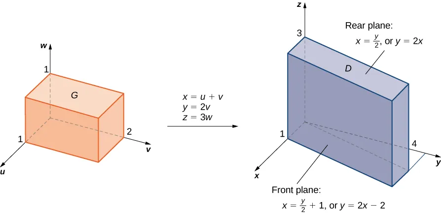
As before, some kind of sketch of the region [latex]G[/latex] in [latex]xyz[/latex]-space over which we have to perform the integration can help identify the region [latex]D[/latex] in [latex]uvw[/latex]-space (Figure 9). Clearly [latex]G[/latex] in [latex]xyz[/latex]-space is bounded by the planes [latex]x=y/2[/latex], [latex]x=(y/2)+1[/latex], [latex]y=0[/latex],[latex]y=4[/latex], [latex]z=0[/latex], and [latex]z=4[/latex]. We also know that we have to use [latex]u=(2x-y)/2[/latex], [latex]v=y/2[/latex] and [latex]w=z/3[/latex] for the transformations. We need to solve for [latex]x[/latex], [latex]y[/latex], and [latex]z[/latex]. Here we find that [latex]x=u+v[/latex], [latex]y=2v[/latex], and [latex]z=3w[/latex].

Using elementary algebra, we can find the corresponding surfaces for the region [latex]G[/latex] and the limits of integration in [latex]uvw[/latex]-space. It is convenient to list these equations in a table.

Equations in [latex]xyz[/latex] for the region [latex]D[/latex]	Corresponding equations in [latex]uvw[/latex] for the region [latex]G[/latex]	Limits for the integration in [latex]uvw[/latex]
[latex]x=y/2[/latex]	[latex]u+v=2v/2=v[/latex]	[latex]u=0[/latex]
[latex]x=y/2[/latex]	[latex]u+v=(2v/2)+1=v+1[/latex]	[latex]u=1[/latex]
[latex]y=0[/latex]	[latex]2v=0[/latex]	[latex]v=0[/latex]
[latex]y=4[/latex]	[latex]2v=4[/latex]	[latex]v=2[/latex]
[latex]z=0[/latex]	[latex]3w=0[/latex]	[latex]w=0[/latex]
[latex]z=3[/latex]	[latex]3w=3[/latex]	[latex]w=1[/latex]

On the left-hand side of this figure, there is a box G with sides 1, 2, and 1 along the u, v, and w axes, respectively. Then there is an arrow from this graph to the right-hand side of the figure marked with x = u + v, y = 2v, and z = 3w. On the right-hand side of this figure there is a region D in xyz space that is a rotated box with sides 1, 4, and 3 along the x, y, and z axes. The rear plane is marked x = y/2 or y = 2x. The front plane is marked x = y/2 + 1 or y = 2x minus 2. — Figure 9. The region [latex]G[/latex] in [latex]uvw[/latex]-space is transformed to region D in [latex]xyz[/latex]-space.

Now we can calculate the Jacobian for the transformation:

[latex]\large{J(u,v,w)=\begin{vmatrix}\frac{\partial{x}}{\partial{u}}&\frac{\partial{x}}{\partial{v}}&\frac{\partial{x}}{\partial{w}} \\ \frac{\partial{y}}{\partial{u}}&\frac{\partial{y}}{\partial{v}}&\frac{\partial{y}}{\partial{w}} \\ \frac{\partial{z}}{\partial{u}}&\frac{\partial{z}}{\partial{v}}&\frac{\partial{z}}{\partial{w}}\end{vmatrix}=\begin{vmatrix}1&1&0 \\ 0&2&0 \\ 0&0&3\end{vmatrix}=6}[/latex].

The function to be integrated becomes

[latex]\large{f(x,y,z)=x+\frac{z}3=u+v+\frac{3w}3=u+v+w}[/latex].

We are now ready to put everything together and complete the problem.

[latex]\hspace{3cm}\large{\begin{align} &\hspace{1cm}\displaystyle\int_0^3\displaystyle\int_0^4\displaystyle\int_{y/2}^{(y/2)+1}\left(x+\frac{z}3\right)dx \ dy \ dz \\ &=\displaystyle\int_0^1\displaystyle\int_0^2\displaystyle\int_0^1(u+v+w)|J(u,v,w)|du \ dv \ dw=\displaystyle\int_0^1\displaystyle\int_0^2\displaystyle\int_0^1(u+v+w)|6|du \ dv \ dw \\ &=6\displaystyle\int_0^1\displaystyle\int_0^2\displaystyle\int_0^1(u+v+w)du \ dv \ dw=6\displaystyle\int_0^1\displaystyle\int_0^2\left[\frac{u^2}2+vu+wu\right]_0^1dv \ dw \\ &=6\displaystyle\int_0^1\displaystyle\int_0^2\left(\frac12+v+w\right)dv \ dw=6\displaystyle\int_0^1\left[\frac12v+\frac{v^2}2+wv\right]_0^2dw \\ &=6\displaystyle\int_0^1(3+2w)dw=6\left[3w+w^2\right]_0^1=24 \end{align}}[/latex].