Gradient
Look back at the formula for the directional derivative: [latex]D_{\bf{u}}f(x,y)=f_x(x,y)\cos\theta+f_y(x,y)\sin\theta[/latex]. The right-hand side can be written as a dot product of two vectors. Define the first vector as [latex]\nabla{f}(x,y)=f_x(x,y){\bf{i}}+f_y(x,y){\bf{j}}[/latex] and the second as [latex]{\bf{u}}=(\cos\theta){\bf{i}}+(\sin\theta){\bf{j}}[/latex]. Then:
[latex]D_{\bf{u}}f(x,y)=\nabla{f}(x,y)\cdot{\bf{u}}[/latex]
The first vector in this equation has a special name: the gradient of the function [latex]f[/latex].
gradient
Let [latex]z=f(x, y)[/latex] be a function of [latex]x[/latex] and [latex]x[/latex] such that [latex]f_x[/latex] and [latex]f_y[/latex] exist. The vector [latex]\nabla{f}(x,y)[/latex] is called the gradient of [latex]f[/latex] and is defined as:
[latex]\nabla{f}(x,y)=f_x(x,y){\bf{i}}+f_y(x,y){\bf{j}}.[/latex]
The vector [latex]\nabla{f}(x,y)[/latex] is also written as “grad [latex]f[/latex]“.
- [latex]f(x,y)=x^2-xy+3y^2[/latex]
- [latex]f(x,y)=\sin{3x}\cos{3y}[/latex]
Properties of the Gradient
The gradient has important properties that make it useful for understanding how functions behave. We’ve already seen one: the formula for the directional derivative. Let’s dig deeper.
Recall that if the angle between two vectors [latex]{\bf{a}}[/latex] and [latex]{\bf{b}}[/latex] is [latex]\varphi[/latex], then [latex]{\bf{a}}\cdot{\bf{b}}=|{\bf{a}}||{\bf{b}}|\cos\varphi[/latex]. If the angle between [latex]\nabla{f}(x_0,y_0)[/latex] and [latex]{\bf{u}}=(\cos\theta){\bf{i}}+(\sin\theta){\bf{j}}[/latex] is [latex]\varphi[/latex], then:
[latex]D_{\bf{u}}f(x_0,y_0)=\nabla{f}(x_0,y_0)\cdot{\bf{u}}=|\nabla{f}(x_0,y_0)||{\bf{u}}|\cos\varphi=|\nabla{f}(x_0,y_0)|\cos\varphi[/latex]
The [latex]|{\bf{u}}|[/latex] term disappears because [latex]{\bf{u}}[/latex] is a unit vector. The directional derivative equals the magnitude of the gradient at [latex](x_0, y_0)[/latex], multiplied by [latex]\cos\varphi[/latex].
Since [latex]\cos\varphi[/latex] ranges from [latex]-1[/latex] to [latex]1[/latex], we can determine when the directional derivative is maximized or minimized:
- If [latex]\varphi=0[/latex], then [latex]\cos\varphi=1[/latex] and [latex]\nabla{f}(x_0,y_0)[/latex] and [latex]{\bf{u}}[/latex] point in the same direction. This maximizes [latex]D_{\bf{u}}f(x_0,y_0)[/latex].
- If [latex]\varphi=\pi[/latex], then [latex]\cos\varphi=-1[/latex] and [latex]\nabla{f}(x_0,y_0)[/latex] and [latex]{\bf{u}}[/latex] point in opposite directions. This minimizes [latex]D_{\bf{u}}f(x_0,y_0)[/latex].
- If [latex]\nabla{f}(x_0,y_0)={\bf{0}}[/latex], then [latex]D_{\bf{u}}f(x_0,y_0)=0[/latex] for any unit vector [latex]{\bf{u}}[/latex].
These cases are outlined in the following theorem.
properties of the gradient
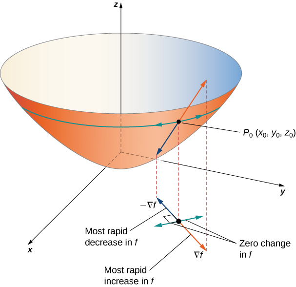
Suppose the function [latex]z=f(x, y)[/latex] is differentiable at [latex](x_0, y_0)[/latex] (Figure 3).
- If [latex]\nabla{f}(x_0,y_0)=0[/latex], then [latex]D_{\bf{u}}f(x_0,y_0)=0[/latex] for any unit vector [latex]\bf{u}[/latex].
- If [latex]\nabla{f}(x_0,y_0)\ne 0[/latex], then [latex]D_{\bf{u}}f(x_0,y_0)[/latex] is maximized when [latex]\bf{u}[/latex] points in the same direction as [latex]\nabla{f}(x_0,y_0)[/latex]. The maximum value of [latex]D_{\bf{u}}f(x_0,y_0)[/latex] is [latex]\|\nabla{f}(x_0,y_0)\|[/latex].
- If [latex]\nabla{f}(x_0,y_0)\ne 0[/latex], then [latex]D_{\bf{u}}f(x_0,y_0)[/latex] is minimized when [latex]\bf{u}[/latex] points in the opposite direction from [latex]\nabla{f}(x_0,y_0)[/latex]. The minimum value of [latex]D_{\bf{u}}f(x_0,y_0)[/latex] is [latex]-\|\nabla{f}(x_0,y_0)\|[/latex].

Interpreting the Gradient
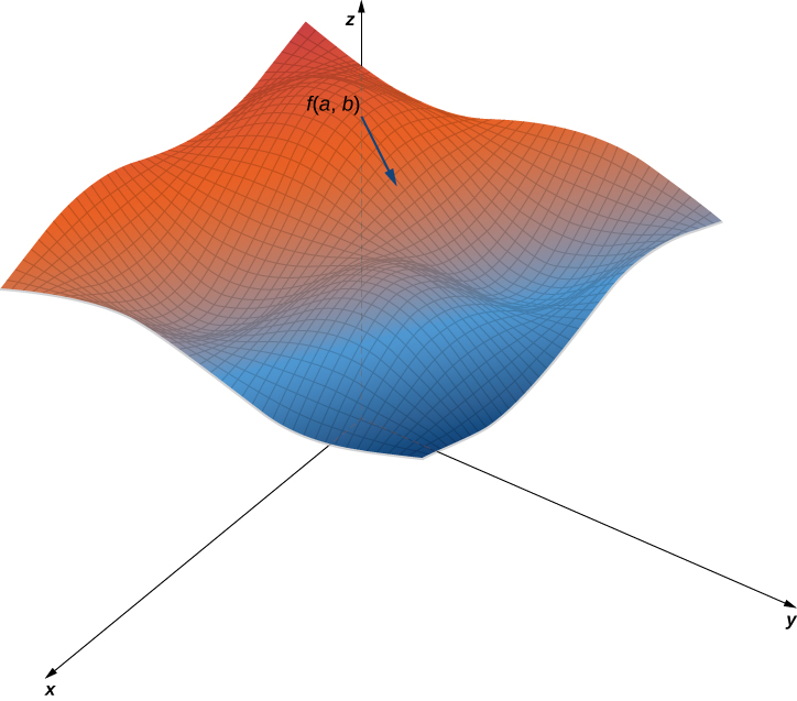
Figure 3 shows part of the graph of [latex]f(x,y)=3+\sin x\sin y[/latex]. Given a point [latex](a, b)[/latex] in the domain of [latex]f[/latex], the maximum value of the gradient at that point is [latex]|\nabla{f}(a,b)|[/latex]. If the surface represented a topographical map, this would be the rate of greatest ascent. In the opposite direction, it would be the rate of greatest descent.
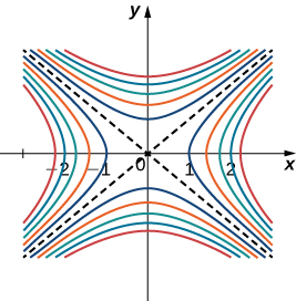
When using a topographical map, the steepest slope is always in the direction where the contour lines are closest together (see Figure 4). This is analogous to the contour map of a function, assuming the level curves are obtained for equally spaced values throughout the range of that function.