We can transform the inside (input values) of a function or we can transform the outside (output values) of a function. Each change has a specific effect that can be seen graphically.
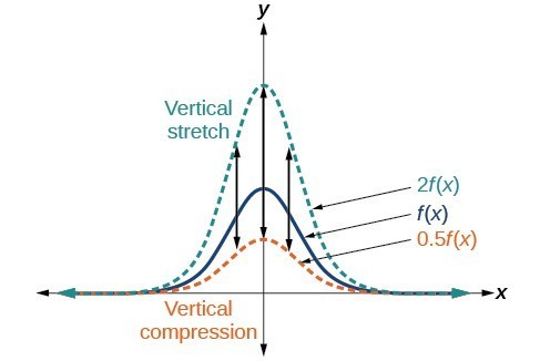
When we multiply a function by a positive constant, we get a function whose graph is stretched or compressed vertically in relation to the graph of the original function. If the constant is greater than 1, we get a vertical stretch; if the constant is between 0 and 1, we get a vertical compression. The graph below shows a function multiplied by constant factors 2 and 0.5 and the resulting vertical stretch and compression.
Vertical stretch and compression
vertical stretches and compressions
A vertical stretch or compression involves scaling the graph of a function [latex]f(x)[/latex] by a constant factor [latex]a[/latex].
[latex]g(x) = a \cdot f(x)[/latex]
This transformation changes the output values of the function.
If [latex]a>1[/latex]: The graph is stretched vertically.
If [latex]0 < a < 1[/latex]: The graph is compressed vertically.
If [latex]a<0[/latex]: A combination of vertical stretch/compression and vertical reflection.
How To: Given a function, graph its vertical stretch.
Identify the value of [latex]a[/latex].
Multiply all range values by [latex]a[/latex].
If [latex]a>1[/latex], the graph is stretched by a factor of [latex]a[/latex].
If [latex]{ 0 }<{ a }<{ 1 }[/latex], the graph is compressed by a factor of [latex]a[/latex].
If [latex]a<0[/latex], the graph is either stretched or compressed and also reflected about the [latex]x[/latex]-axis.
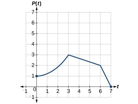
A function [latex]P\left(t\right)[/latex] models the number of fruit flies in a population over time, and is graphed below.A scientist is comparing this population to another population, [latex]Q[/latex], whose growth follows the same pattern, but is twice as large. Sketch a graph of this population.
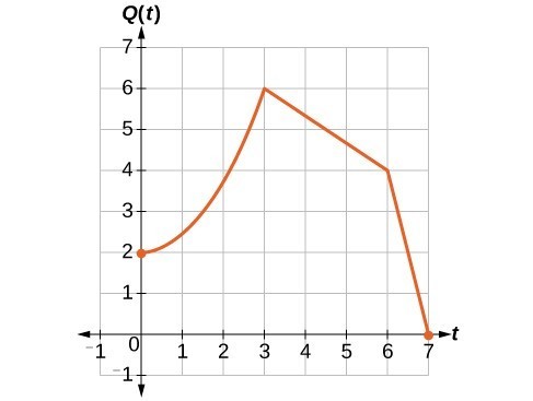
Because the population is always twice as large, the new population’s output values are always twice the original function’s output values.If we choose four reference points, [latex](0, 1)[/latex], [latex](3, 3)[/latex], [latex](6, 2)[/latex] and [latex](7, 0)[/latex] we will multiply all of the outputs by [latex]2[/latex].The following shows where the new points for the new graph will be located.
This means that for any input [latex]t[/latex], the value of the function [latex]Q[/latex] is twice the value of the function [latex]P[/latex]. Notice that the effect on the graph is a vertical stretching of the graph, where every point doubles its distance from the horizontal axis. The input values, [latex]t[/latex], stay the same while the output values are twice as large as before.
A function [latex]f[/latex] is given in the table below. Create a table for the function [latex]g\left(x\right)=\frac{1}{2}f\left(x\right)[/latex].
[latex]x[/latex]
[latex]2[/latex]
[latex]4[/latex]
[latex]6[/latex]
[latex]8[/latex]
[latex]f\left(x\right)[/latex]
[latex]1[/latex]
[latex]3[/latex]
[latex]7[/latex]
[latex]11[/latex]
The formula [latex]g\left(x\right)=\frac{1}{2}f\left(x\right)[/latex] tells us that the output values of [latex]g[/latex] are half of the output values of [latex]f[/latex] with the same inputs. For example, we know that [latex]f\left(4\right)=3[/latex]. Then:
We do the same for the other values to produce this table.
[latex]x[/latex]
[latex]2[/latex]
[latex]4[/latex]
[latex]6[/latex]
[latex]8[/latex]
[latex]g\left(x\right)[/latex]
[latex]\frac{1}{2}[/latex]
[latex]\frac{3}{2}[/latex]
[latex]\frac{7}{2}[/latex]
[latex]\frac{11}{2}[/latex]
[latex]\\[/latex] Analysis of the Solution
The result is that the function [latex]g\left(x\right)[/latex] has been compressed vertically by [latex]\frac{1}{2}[/latex]. Each output value is divided in half, so the graph is half the original height.
Horizontal Stretches and Compressions
Now we consider changes to the inside of a function. When we multiply a function’s input by a positive constant, we get a function whose graph is stretched or compressed horizontally in relation to the graph of the original function. If the constant is between 0 and 1, we get a horizontal stretch; if the constant is greater than 1, we get a horizontal compression of the function.
Given a function [latex]y=f\left(x\right)[/latex], the form [latex]y=f\left(bx\right)[/latex] results in a horizontal stretch or compression. Consider the function [latex]y={x}^{2}[/latex]. The graph of [latex]y={\left(0.5x\right)}^{2}[/latex] is a horizontal stretch of the graph of the function [latex]y={x}^{2}[/latex] by a factor of 2. The graph of [latex]y={\left(2x\right)}^{2}[/latex] is a horizontal compression of the graph of the function [latex]y={x}^{2}[/latex] by a factor of [latex]2[/latex].
horizontal stretches and compressions
A horizontal stretch or compression involves scaling the graph of a function [latex]f(x)[/latex] by a constant factor [latex]b[/latex].
[latex]g(x) = f(b \cdot x)[/latex]
This transformation changes the input values of the function.
If [latex]b>1[/latex]: The graph is compressed horizontally. The graph is compressed by [latex]\dfrac{1}{b}[/latex].
If [latex]0 < b < 1[/latex]: The graph is stretched horizontally. The graph is stretched by [latex]\dfrac{1}{b}[/latex].
If [latex]b<0[/latex]: A combination of horizontal stretch/compression and horizontal reflection.
Suppose a scientist is comparing a population of fruit flies to a population that progresses through its lifespan twice as fast as the original population. In other words, this new population, [latex]R[/latex], will progress in [latex]1[/latex] hour the same amount as the original population does in [latex]2[/latex] hours, and in [latex]2[/latex] hours, it will progress as much as the original population does in [latex]4[/latex] hours. Sketch a graph of this population.
Symbolically, we could write
[latex]\begin{align}&R\left(1\right)=P\left(2\right), \\ &R\left(2\right)=P\left(4\right),\text{ and in general,} \\ &R\left(t\right)=P\left(2t\right). \end{align}[/latex]
See below for a graphical comparison of the original population and the compressed population.
(a) Original population graph (b) Compressed population graph
[latex]\\[/latex] Analysis of the Solution
[latex]\\[/latex]
Note that the effect on the graph is a horizontal compression where all input values are half of their original distance from the vertical axis.
A function [latex]f\left(x\right)[/latex] is given below. Create a table for the function [latex]g\left(x\right)=f\left(\frac{1}{2}x\right)[/latex].
[latex]x[/latex]
[latex]2[/latex]
[latex]4[/latex]
[latex]6[/latex]
[latex]8[/latex]
[latex]f\left(x\right)[/latex]
[latex]1[/latex]
[latex]3[/latex]
[latex]7[/latex]
[latex]11[/latex]
The formula [latex]g\left(x\right)=f\left(\frac{1}{2}x\right)[/latex] tells us that the output values for [latex]g[/latex] are the same as the output values for the function [latex]f[/latex] at an input half the size. Notice that we do not have enough information to determine [latex]g\left(2\right)[/latex] because [latex]g\left(2\right)=f\left(\frac{1}{2}\cdot 2\right)=f\left(1\right)[/latex], and we do not have a value for [latex]f\left(1\right)[/latex] in our table. Our input values to [latex]g[/latex] will need to be twice as large to get inputs for [latex]f[/latex] that we can evaluate. For example, we can determine [latex]g\left(4\right)\text{.}[/latex]
We do the same for the other values to produce the table below.
[latex]x[/latex]
4
8
12
16
[latex]g\left(x\right)[/latex]
1
3
7
11
This figure shows the graphs of both of these sets of points.
Analysis of the Solution
Because each input value has been doubled, the result is that the function [latex]g\left(x\right)[/latex] has been stretched horizontally by a factor of 2.
 Symbolically, the relationship is written as
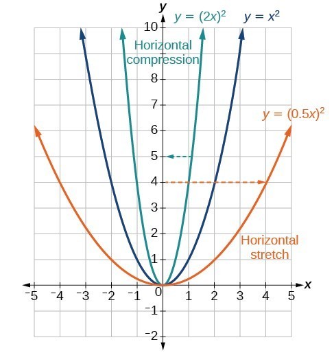
![Two side-by-side graphs. The first graph has function for original population whose domain is [0,7] and range is [0,3]. The maximum value occurs at (3,3). The second graph has the same shape as the first except it is half as wide. It is a graph of transformed population, with a domain of [0, 3.5] and a range of [0,3]. The maximum occurs at (1.5, 3).](https://s3-us-west-2.amazonaws.com/courses-images/wp-content/uploads/sites/896/2016/10/18203623/CNX_Precalc_Figure_01_05_029ab.jpg)
