• Find the average rate of change
• Use a graph to see where a function is going up, going down, or staying flat
• Use a graph to identify the highest and lowest points

Climate Research Station

In calculus, you’ll use derivatives to find exact rates of change at any instant, locate precise extrema, and solve optimization problems. Today’s work with average rates and graphical analysis builds the foundation for these calculus tools.

A climate station recorded atmospheric CO₂ levels over a 10-year period:

Year	2014	2016	2018	2020	2022	2024
CO₂ (ppm)	398.7	404.2	408.5	414.1	421.0	424.3

Average rate of change is calculated as [latex]\frac{f(b)-f(a)}{b-a}[/latex]​

But what was the rate of change in 2014? In calculus, we’ll learn to extend the average rate of change and find the instantaneous rate of change at any specific moment using derivatives, giving us more precise information than these averages.

The NOAA Mauna Loa Observatory (MLO) is a key atmospheric research facility that monitors and collects long-term data on atmospheric composition and climate change. It’s known for its continuous measurements of rising carbon dioxide (CO2) concentrations, ozone, and other atmospheric constituents. The data collected at MLO helps scientists understand the impacts of human activities on the atmosphere and climate.

---

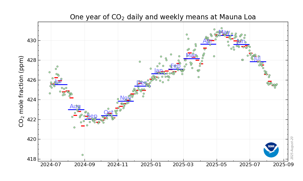
Your station models the annual CO₂ cycle with: [latex]C(d) = 426 + 3.85sin(\frac{2π}{365}(d-105))[/latex] where d = day of year.

This function captures how CO₂ levels fluctuate seasonally – rising in winter when plants are dormant and falling in summer when photosynthesis is most active.

CO₂ monitoring is crucial for understanding our climate and how it may be changing over time. Learn more about the NOAA: https://gml.noaa.gov/about/networks.html