Consider sets of equations given by [latex]x\left(t\right)[/latex] and [latex]y\left(t\right)[/latex] where [latex]t[/latex] is the independent variable of time. We can use these parametric equations in a number of applications when we are looking for not only a particular position but also the direction of the movement. As we trace out successive values of [latex]t[/latex], the orientation of the curve becomes clear. This is one of the primary advantages of using parametric equations: we are able to trace the movement of an object along a path according to time.

Parameterizing a Curve

When an object moves along a curve—or curvilinear path—in a given direction and in a given amount of time, the position of the object in the plane is given by the x-coordinate and the y-coordinate. However, both [latex]x[/latex] and [latex]y[/latex] vary over time and so are functions of time. For this reason, we add another variable, the parameter, upon which both [latex]x[/latex] and [latex]y[/latex] are dependent functions. Parametric equations primarily describe motion and direction.

parameter

The variable that [latex]x[/latex] and [latex]y[/latex] are both dependent on.

When we parameterize a curve, we are translating a single equation in two variables, such as [latex]x[/latex] and [latex]y[/latex], into an equivalent pair of equations in three variables, [latex]x,y[/latex], and [latex]t[/latex]. One of the reasons we parameterize a curve is because the parametric equations yield more information: specifically, the direction of the object’s motion over time.

When we graph parametric equations, we can observe the individual behaviors of [latex]x[/latex] and of [latex]y[/latex]. There are a number of shapes that cannot be represented in the form [latex]y=f\left(x\right)[/latex], meaning that they are not functions. For example, consider the graph of a circle, given as [latex]{r}^{2}={x}^{2}+{y}^{2}[/latex]. Solving for [latex]y[/latex] gives [latex]y=\pm \sqrt{{r}^{2}-{x}^{2}}[/latex], or two equations: [latex]{y}_{1}=\sqrt{{r}^{2}-{x}^{2}}[/latex] and [latex]{y}_{2}=-\sqrt{{r}^{2}-{x}^{2}}[/latex]. If we graph [latex]{y}_{1}[/latex] and [latex]{y}_{2}[/latex] together, the graph will not pass the vertical line test. Thus, the equation for the graph of a circle is not a function.

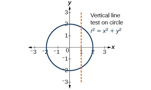
However, if we were to graph each equation on its own, each one would pass the vertical line test and therefore would represent a function. In some instances, the concept of breaking up the equation for a circle into two functions is similar to the concept of creating parametric equations, as we use two functions to produce a non-function. This will become clearer as we move forward.

parametric equations

Suppose [latex]t[/latex] is a number on an interval, [latex]I[/latex]. The set of ordered pairs, [latex]\left(x\left(t\right),y\left(t\right)\right)[/latex], where [latex]x=f\left(t\right)[/latex] and [latex]y=g\left(t\right)[/latex], forms a plane curve based on the parameter [latex]t[/latex]. The equations [latex]x=f\left(t\right)[/latex] and [latex]y=g\left(t\right)[/latex] are the parametric equations.

Parameterize the curve [latex]y={x}^{2}-1[/latex] letting [latex]x\left(t\right)=t[/latex]. Graph both equations.

Show Solution

If [latex]x\left(t\right)=t[/latex], then to find [latex]y\left(t\right)[/latex] we replace the variable [latex]x[/latex] with the expression given in [latex]x\left(t\right)[/latex]. In other words, [latex]y\left(t\right)={t}^{2}-1[/latex]. Make a table of values similar to the table below, and sketch the graph.

[latex]t[/latex]	[latex]x\left(t\right)[/latex]	[latex]y\left(t\right)[/latex]
[latex]-4[/latex]	[latex]-4[/latex]	[latex]y\left(-4\right)={\left(-4\right)}^{2}-1=15[/latex]
[latex]-3[/latex]	[latex]-3[/latex]	[latex]y\left(-3\right)={\left(-3\right)}^{2}-1=8[/latex]
[latex]-2[/latex]	[latex]-2[/latex]	[latex]y\left(-2\right)={\left(-2\right)}^{2}-1=3[/latex]
[latex]-1[/latex]	[latex]-1[/latex]	[latex]y\left(-1\right)={\left(-1\right)}^{2}-1=0[/latex]
[latex]0[/latex]	[latex]0[/latex]	[latex]y\left(0\right)={\left(0\right)}^{2}-1=-1[/latex]
[latex]1[/latex]	[latex]1[/latex]	[latex]y\left(1\right)={\left(1\right)}^{2}-1=0[/latex]
[latex]2[/latex]	[latex]2[/latex]	[latex]y\left(2\right)={\left(2\right)}^{2}-1=3[/latex]
[latex]3[/latex]	[latex]3[/latex]	[latex]y\left(3\right)={\left(3\right)}^{2}-1=8[/latex]
[latex]4[/latex]	[latex]4[/latex]	[latex]y\left(4\right)={\left(4\right)}^{2}-1=15[/latex]

It may be helpful to use the TRACE feature of a graphing calculator to see how the points are generated as [latex]t[/latex] increases.

Analysis of the SolutionThe arrows indicate the direction in which the curve is generated. Notice the curve is identical to the curve of [latex]y={x}^{2}-1[/latex].

Construct a table of values and plot the parametric equations: [latex]x\left(t\right)=t - 3,y\left(t\right)=2t+4;-1\le t\le 2[/latex].

Show Solution

[latex]t[/latex]	[latex]x\left(t\right)[/latex]	[latex]y\left(t\right)[/latex]
[latex]-1[/latex]	[latex]-4[/latex]	[latex]2[/latex]
[latex]0[/latex]	[latex]-3[/latex]	[latex]4[/latex]
[latex]1[/latex]	[latex]-2[/latex]	[latex]6[/latex]
[latex]2[/latex]	[latex]-1[/latex]	[latex]8[/latex]