While translating from polar coordinates to Cartesian coordinates may seem simpler in some instances, graphing the classic curves is actually less complicated in the polar system. The next curve is called a cardioid, as it resembles a heart. This shape is often included with the family of curves called limaçons, but here we will discuss the cardioid on its own.
cardiods
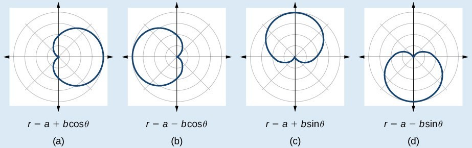
The formulas that produce the graphs of a cardioid are given by [latex]r=a\pm b\cos \theta[/latex] and [latex]r=a\pm b\sin \theta[/latex] where [latex]a>0,b>0[/latex], and [latex]\frac{a}{b}=1[/latex]. The cardioid graph passes through the pole.
How To: Given the polar equation of a cardioid, sketch its graph.
Check equation for the three types of symmetry.
Find the zeros. Set [latex]r=0[/latex].
Find the maximum value of the equation according to the maximum value of the trigonometric expression.
Make a table of values for [latex]r[/latex] and [latex]\theta[/latex].
Plot the points and sketch the graph.
Sketch the graph of [latex]r=2+2\cos \theta[/latex].
First, testing the equation for symmetry, we find that the graph of this equation will be symmetric about the polar axis. Next, we find the zeros and maximums. Setting [latex]r=0[/latex], we have [latex]\theta =\pi +2k\pi[/latex]. The zero of the equation is located at [latex]\left(0,\pi \right)[/latex]. The graph passes through this point.
The maximum value of [latex]r=2+2\cos \theta[/latex] occurs when [latex]\cos \theta[/latex] is a maximum, which is when [latex]\cos \theta =1[/latex] or when [latex]\theta =0[/latex]. Substitute [latex]\theta =0[/latex] into the equation, and solve for [latex]r[/latex].
The point [latex]\left(4,0\right)[/latex] is the maximum value on the graph.
We found that the polar equation is symmetric with respect to the polar axis, but as it extends to all four quadrants, we need to plot values over the interval [latex]\left[0,\pi \right][/latex]. The upper portion of the graph is then reflected over the polar axis. Next, we make a table of values, as in the table below, and then we plot the points and draw the graph. See Figure 8.