To graph in the rectangular coordinate system we construct a table of [latex]x[/latex] and [latex]y[/latex] values. To graph in the polar coordinate system we construct a table of [latex]\theta[/latex] and [latex]r[/latex] values. We enter values of [latex]\theta[/latex] into a polar equation and calculate [latex]r[/latex]. However, using the properties of symmetry and finding key values of [latex]\theta[/latex] and [latex]r[/latex] means fewer calculations will be needed.
Finding Zeros and Maxima
To find the zeros of a polar equation, we solve for the values of [latex]\theta[/latex] that result in [latex]r=0[/latex]. Recall that, to find the zeros of polynomial functions, we set the equation equal to zero and then solve for [latex]x[/latex]. We use the same process for polar equations. Set [latex]r=0[/latex], and solve for [latex]\theta[/latex].
For many of the forms we will encounter, the maximum value of a polar equation is found by substituting those values of [latex]\theta[/latex] into the equation that result in the maximum value of the trigonometric functions. Consider [latex]r=5\cos \theta[/latex]; the maximum distance between the curve and the pole is 5 units. The maximum value of the cosine function is 1 when [latex]\theta =0[/latex], so our polar equation is [latex]5\cos \theta[/latex], and the value [latex]\theta =0[/latex] will yield the maximum [latex]|r|[/latex].
Similarly, the maximum value of the sine function is 1 when [latex]\theta =\frac{\pi }{2}[/latex], and if our polar equation is [latex]r=5\sin \theta[/latex], the value [latex]\theta =\frac{\pi }{2}[/latex] will yield the maximum [latex]|r|[/latex]. We may find additional information by calculating values of [latex]r[/latex] when [latex]\theta =0[/latex]. These points would be polar axis intercepts, which may be helpful in drawing the graph and identifying the curve of a polar equation.
Find the zeros and maximum [latex]|r|[/latex] and, if necessary, the polar axis intercepts of [latex]r=2\sin \theta[/latex].
To find the zeros, set [latex]r[/latex] equal to zero and solve for [latex]\theta[/latex].
[latex]\begin{align}&2\sin \theta =0 \\ &\sin \theta =0 \\ &\theta ={\sin }^{-1}0 \\ &\theta =n\pi&& \text{where }n\text{ is an integer} \end{align}[/latex]
Substitute any one of the [latex]\theta[/latex] values into the equation. We will use [latex]0[/latex].
The points [latex]\left(0,0\right)[/latex] and [latex]\left(0,\pm n\pi \right)[/latex] are the zeros of the equation. They all coincide, so only one point is visible on the graph. This point is also the only polar axis intercept.
To find the maximum value of the equation, look at the maximum value of the trigonometric function [latex]\sin \theta[/latex], which occurs when [latex]\theta =\frac{\pi }{2}\pm 2k\pi[/latex] resulting in [latex]\sin \left(\frac{\pi }{2}\right)=1[/latex]. Substitute [latex]\frac{\pi }{2}[/latex] for [latex]\mathrm{\theta .}[/latex]
The point [latex]\left(2,\frac{\pi }{2}\right)[/latex] will be the maximum value on the graph. Let’s plot a few more points to verify the graph of a circle.
Without converting to Cartesian coordinates, test the given equation for symmetry and find the zeros and maximum values of [latex]|r|:[/latex] [latex]r=3\cos \theta[/latex].
Tests will reveal symmetry about the polar axis. The zero is [latex]\left(0,\frac{\pi }{2}\right)[/latex], and the maximum value is [latex]\left(3,0\right)[/latex].
Graphing Circles and the Classic Polar Curves
Investigating Circles
Now we have seen the equation of a circle in the polar coordinate system. In the last two examples, the same equation was used to illustrate the properties of symmetry and demonstrate how to find the zeros, maximum values, and plotted points that produced the graphs. However, the circle is only one of many shapes in the set of polar curves.
There are five classic polar curves: cardioids, limaҫons, lemniscates, rose curves, and Archimedes’ spirals. We will briefly touch on the polar formulas for the circle before moving on to the classic curves and their variations.
circles in polar form
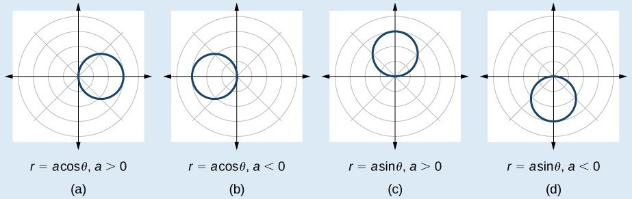
Some of the formulas that produce the graph of a circle in polar coordinates are given by [latex]r=a\cos \theta[/latex] and [latex]r=a\sin \theta[/latex], where [latex]a[/latex] is the diameter of the circle or the distance from the pole to the farthest point on the circumference. The radius is [latex]\frac{|a|}{2}[/latex], or one-half the diameter. For [latex]r=a\cos \theta ,[/latex] the center is [latex]\left(\frac{a}{2},0\right)[/latex]. For [latex]r=a\sin \theta[/latex], the center is [latex]\left(\frac{a}{2},\pi \right)[/latex].
Sketch the graph of [latex]r=4\cos \theta[/latex].
First, testing the equation for symmetry, we find that the graph is symmetric about the polar axis. Next, we find the zeros and maximum [latex]|r|[/latex] for [latex]r=4\cos \theta[/latex]. First, set [latex]r=0[/latex], and solve for [latex]\theta[/latex] . Thus, a zero occurs at [latex]\theta =\frac{\pi }{2}\pm k\pi[/latex]. A key point to plot is [latex]\left(0,\text{ }\text{ }\frac{\pi }{2}\right)[/latex].To find the maximum value of [latex]r[/latex], note that the maximum value of the cosine function is 1 when [latex]\theta =0\pm 2k\pi[/latex]. Substitute [latex]\theta =0[/latex] into the equation:
The maximum value of the equation is 4. A key point to plot is [latex]\left(4,0\right)[/latex].
As [latex]r=4\cos \theta[/latex] is symmetric with respect to the polar axis, we only need to calculate r-values for [latex]\theta[/latex] over the interval [latex]\left[0,\pi \right][/latex]. Points in the upper quadrant can then be reflected to the lower quadrant. Make a table of values similar to the table below.
[latex]\theta[/latex]
0
[latex]\frac{\pi }{6}[/latex]
[latex]\frac{\pi }{4}[/latex]
[latex]\frac{\pi }{3}[/latex]
[latex]\frac{\pi }{2}[/latex]
[latex]\frac{2\pi }{3}[/latex]
[latex]\frac{3\pi }{4}[/latex]
[latex]\frac{5\pi }{6}[/latex]
[latex]\pi[/latex]
[latex]r[/latex]
4
3.46
2.83
2
0
−2
−2.83
−3.46
4
Create a table of values for r = 4sin θ using θ values: 0, π/6, π/2, π, and determine what type of curve this represents.When you see [latex]r = a\cos \theta[/latex] or [latex]r = a\sin \theta[/latex], you can immediately recognize these as circles without plotting every point. The cosine version creates a circle centered on the positive x-axis, while the sine version creates a circle centered on the positive y-axis.