A car’s speedometer shows instantaneous speed—how fast you’re traveling at a specific moment. But how do we calculate instantaneous velocity from position data? Limits provide the answer by examining what happens as time intervals become infinitesimally small.
Average velocity over an interval is calculated as [latex]\frac{\text{change in position}}{\text{change in time}}[/latex].
Instantaneous velocity is found by taking the limit as the time interval approaches zero—this is the foundation of derivatives in calculus.
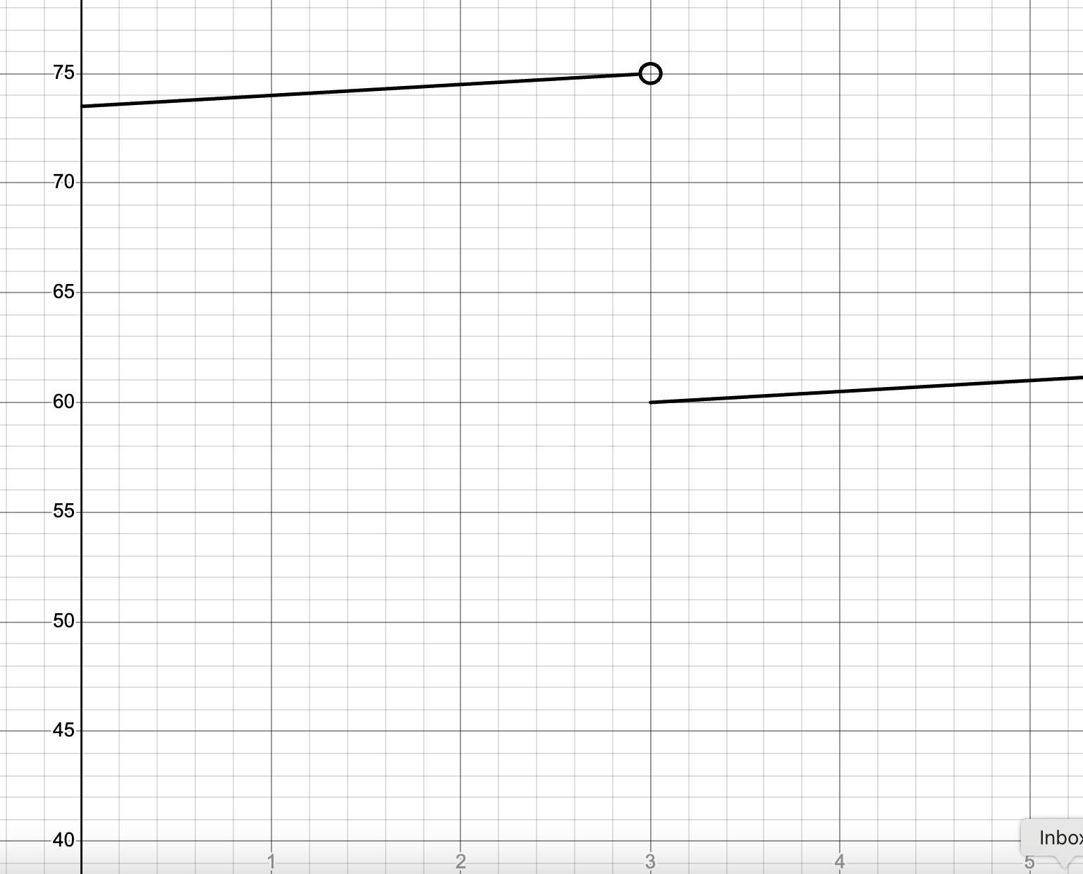
A factory monitors the temperature [latex]T(t)[/latex] in degrees Celsius of a chemical reaction over time [latex]t[/latex] in minutes. The graph shows the temperature function with a break at [latex]t = 3[/latex] minutes when operators adjust the reaction conditions.
Use the graph to find:
a) [latex]\lim_{t \to 3^-} T(t)[/latex]
b) [latex]\lim_{t \to 3^+} T(t)[/latex]
c) [latex]\lim_{t \to 3} T(t)[/latex]
d) [latex]T(3)[/latex]
a) Left-hand limit: As [latex]t[/latex] approaches 3 from the left ([latex]t < 3[/latex]), we observe the branch of the graph to the left of [latex]t = 3[/latex]. The temperature values approach 75°C. [latex]\lim_{t \to 3^-} T(t) = 75[/latex]
b) Right-hand limit: As [latex]t[/latex] approaches 3 from the right ([latex]t > 3[/latex]), we observe the branch to the right of [latex]t = 3[/latex]. The temperature values approach 60°C. [latex]\lim_{t \to 3^+} T(t) = 60[/latex]
c) Two-sided limit: Since the left-hand limit (75) does not equal the right-hand limit (60), the two-sided limit does not exist. [latex]\lim_{t \to 3} T(t) \text{ does not exist}[/latex]
d) Function value: The filled circle at [latex](3, 60)[/latex] indicates the actual temperature at [latex]t = 3[/latex]. [latex]T(3) = 60[/latex]°C
A limit can exist even when the function value doesn’t, and a function value can exist even when the limit doesn’t! The limit only cares about what’s happening near the point, not at the point.A population biologist models bacterial growth with the function [latex]f(x) = \frac{x^3 - 125}{x - 5}[/latex], where [latex]x[/latex] represents hours after midnight. Estimate [latex]\lim_{x \to 5} f(x)[/latex] using a table of values.
Notice that [latex]f(5)[/latex] is undefined because substituting [latex]x = 5[/latex] gives [latex]\frac{0}{0}[/latex]. However, we can still find the limit by examining values near 5. Let’s create a table with values approaching 5 from both sides: [latex]x[/latex] (from left) [latex]f(x)[/latex] [latex]x[/latex] (from right) [latex]f(x)[/latex] 4.9 73.51 5.1 76.51 4.99 74.8501 5.01 75.1501 4.999 74.985 5.001 75.015 4.9999 74.9985 5.0001 75.0015 Analysis: As [latex]x[/latex] approaches 5 from the left, [latex]f(x)[/latex] approaches 75. As [latex]x[/latex] approaches 5 from the right, [latex]f(x)[/latex] approaches 75. Since both one-sided limits equal 75: [latex]\lim_{x \to 5} f(x) = 75[/latex] Even though [latex]f(5)[/latex] doesn’t exist, the bacterial population model predicts the population is approaching a value corresponding to 75 at the 5-hour mark.
A ball is dropped from a height, and the function [latex]h(t) = \dfrac{5t^{2}-3t+2}{t-1}[/latex] models the height of the ball (in meters) at time [latex]t[/latex] seconds, except when [latex]t=1[/latex].
Use a table of values to estimate [latex]\displaystyle \lim_{t\to 1} h(t)[/latex].
t
0.9
0.95
0.99
1.01
1.05
1.1
h(t)
Estimate the value that [latex]h(t)[/latex] approaches as [latex]t[/latex] gets closer to 1.