- Graph linear functions using a table of values.
- Identify and interpret the slope and intercepts of a linear function.
- Write the equation for a linear function from the graph of a line.
Graphing a Linear Function Using Transformations
Another option for graphing is to use transformations of the identity function [latex]f(x)=x[/latex] . A function may be transformed by a shift up, down, left, or right. A function may also be transformed using a reflection, stretch, or compression.
Vertical Stretch or Compression
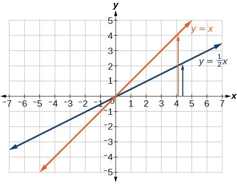
In the equation [latex]f(x)=mx[/latex], the m is acting as the vertical stretch or compression of the identity function. When m is negative, there is also a vertical reflection of the graph. Notice in Figure 4 that multiplying the equation of [latex]f(x)=x[/latex] by m stretches the graph of f by a factor of m units if m > 1 and compresses the graph of f by a factor of m units if 0 < m < 1. This means the larger the absolute value of m, the steeper the slope.
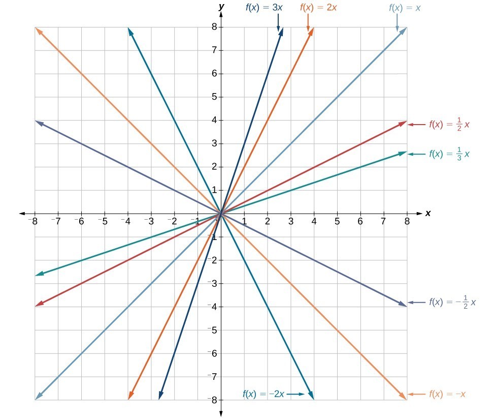
Figure 4. Vertical stretches and compressions and reflections on the function [latex]f\left(x\right)=x[/latex].
Vertical Shift
In [latex]f\left(x\right)=mx+b[/latex], the b acts as the vertical shift, moving the graph up and down without affecting the slope of the line. Notice in Figure 5 that adding a value of b to the equation of [latex]f\left(x\right)=x[/latex] shifts the graph of f a total of b units up if b is positive and |b| units down if b is negative.
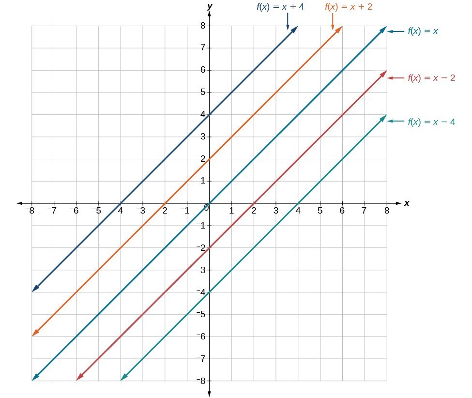
Figure 5. This graph illustrates vertical shifts of the function [latex]f(x)=x[/latex].
Using vertical stretches or compressions along with vertical shifts is another way to look at identifying different types of linear functions. Although this may not be the easiest way to graph this type of function, it is still important to practice each method.
How To: Given the equation of a linear function, use transformations to graph the linear function in the form [latex]f\left(x\right)=mx+b[/latex].
- Graph [latex]f\left(x\right)=x[/latex].
- Vertically stretch or compress the graph by a factor m.
- Shift the graph up or down b units.
Example 3: Graphing by Using Transformations
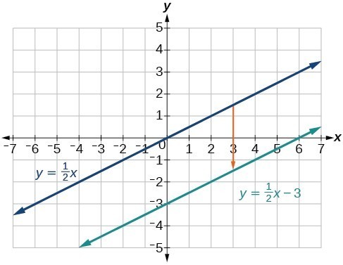
Graph [latex]f\left(x\right)=\frac{1}{2}x - 3[/latex] using transformations.
Graph [latex]f\left(x\right)=4+2x[/latex], using transformations.

Q & A
In Example 3, could we have sketched the graph by reversing the order of the transformations?
No. The order of the transformations follows the order of operations. When the function is evaluated at a given input, the corresponding output is calculated by following the order of operations. This is why we performed the compression first. For example, following the order: Let the input be 2.
Writing the Equation for a Function from the Graph of a Line
Recall that in Linear Functions, we wrote the equation for a linear function from a graph. Now we can extend what we know about graphing linear functions to analyze graphs a little more closely. Begin by taking a look at Figure 8. We can see right away that the graph crosses the y-axis at the point (0, 4) so this is the y-intercept.
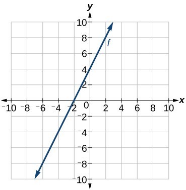
Then we can calculate the slope by finding the rise and run. We can choose any two points, but let’s look at the point (–2, 0). To get from this point to the y-intercept, we must move up 4 units (rise) and to the right 2 units (run). So the slope must be
Substituting the slope and y-intercept into the slope-intercept form of a line gives
How To: Given a graph of linear function, find the equation to describe the function.
- Identify the y-intercept of an equation.
- Choose two points to determine the slope.
- Substitute the y-intercept and slope into the slope-intercept form of a line.
Example 4: Matching Linear Functions to Their Graphs
Figure 10[/hidden-answer]
Finding the x-intercept of a Line
So far, we have been finding the y-intercepts of a function: the point at which the graph of the function crosses the y-axis. A function may also have an x-intercept, which is the x-coordinate of the point where the graph of the function crosses the x-axis. In other words, it is the input value when the output value is zero.
To find the x-intercept, set a function f(x) equal to zero and solve for the value of x. For example, consider the function shown.
Set the function equal to 0 and solve for x.
The graph of the function crosses the x-axis at the point (2, 0).
Q & A
Do all linear functions have x-intercepts?
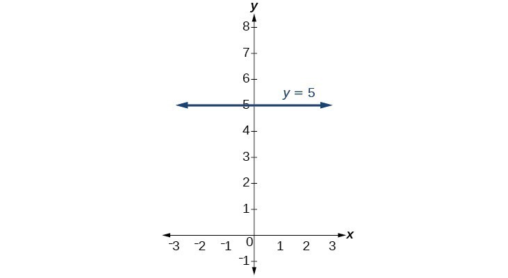
No. However, linear functions of the form y = c, where c is a nonzero real number are the only examples of linear functions with no x-intercept. For example, y = 5 is a horizontal line 5 units above the x-axis. This function has no x-intercepts.
A General Note: x-intercept
The x-intercept of the function is the point where the graph crosses the x-axis. Points on the x-axis have the form (x,0) so we can find x-intercepts by setting f(x) = 0. For a linear function, we solve the equation mx + b = 0
Example 5: Finding an x-intercept
Find the x-intercept of [latex]f\left(x\right)=\frac{1}{2}x - 3[/latex].
Find the x-intercept of [latex]f\left(x\right)=\frac{1}{4}x - 4[/latex].
Calculating and Interpreting Slope
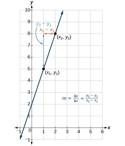
In the examples we have seen so far, we have had the slope provided for us. However, we often need to calculate the slope given input and output values. Given two values for the input, [latex]{x}_{1}[/latex] and [latex]{x}_{2}[/latex], and two corresponding values for the output, [latex]{y}_{1}[/latex] and [latex]{y}_{2}[/latex] —which can be represented by a set of points, [latex]\left({x}_{1}\text{, }{y}_{1}\right)[/latex] and [latex]\left({x}_{2}\text{, }{y}_{2}\right)[/latex]—we can calculate the slope [latex]m[/latex], as follows
where [latex]\Delta y[/latex] is the vertical displacement and [latex]\Delta x[/latex] is the horizontal displacement. Note in function notation two corresponding values for the output [latex]{y}_{1}[/latex] and [latex]{y}_{2}[/latex] for the function [latex]f[/latex], [latex]{y}_{1}=f\left({x}_{1}\right)[/latex] and [latex]{y}_{2}=f\left({x}_{2}\right)[/latex], so we could equivalently write
The graph in Figure 5 indicates how the slope of the line between the points, [latex]\left({x}_{1,}{y}_{1}\right)[/latex]
and [latex]\left({x}_{2,}{y}_{2}\right)[/latex], is calculated. Recall that the slope measures steepness. The greater the absolute value of the slope, the steeper the line is.
The slope of a function is calculated by the change in [latex]y[/latex]
Finding the Slope of a Linear Function
If [latex]f\left(x\right)[/latex] is a linear function, and [latex]\left(3,-2\right)[/latex] and [latex]\left(8,1\right)[/latex] are points on the line, find the slope. Is this function increasing or decreasing?
If [latex]f\left(x\right)[/latex] is a linear function, and [latex]\left(2,\text{ }3\right)[/latex] and [latex]\left(0,\text{ }4\right)[/latex] are points on the line, find the slope. Is this function increasing or decreasing?
Example 4: Finding the Population Change from a Linear Function
The population of a city increased from 23,400 to 27,800 between 2008 and 2012. Find the change of population per year if we assume the change was constant from 2008 to 2012.
Analysis of the Solution
A graph of the function is shown in Figure 12. We can see that the x-intercept is (6, 0) as we expected.