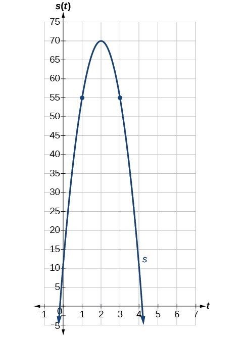
Many applications of the derivative involve determining the rate of change at a given instant of a function with the independent variable time—which is why the term instantaneous is used. Consider the height of a ball tossed upward with an initial velocity of 64 feet per second, given by [latex]s\left(t\right)=-16{t}^{2}+64t+6[/latex], where [latex]t[/latex] is measured in seconds and [latex]s\left(t\right)[/latex] is measured in feet. We know the path is that of a parabola. The derivative will tell us how the height is changing at any given point in time. The height of the ball is shown as a function of time. In physics, we call this the “s–t graph.”
Using the function, [latex]s\left(t\right)=-16{t}^{2}+64t+6[/latex], what is the instantaneous velocity of the ball at 1 second and 3 seconds into its flight?
The velocity at [latex]t=1[/latex] and [latex]t=3[/latex] is the instantaneous rate of change of distance per time, or velocity. Notice that the initial height is 6 feet. To find the instantaneous velocity, we find the derivative and evaluate it at [latex]t=1[/latex] and [latex]t=3:[/latex]
[latex]\begin{align}{f}^{\prime }\left(a\right)&=\underset{h\to 0}{\mathrm{lim}}\frac{f\left(a+h\right)-f\left(a\right)}{h} \\ &=\underset{h\to 0}{\mathrm{lim}}\frac{-16{\left(t+h\right)}^{2}+64\left(t+h\right)+6-\left(-16{t}^{2}+64t+6\right)}{h}&& \text{Substitute }s\left(t+h\right)\text{ and }s\left(t\right). \\ &=\underset{h\to 0}{\mathrm{lim}}\frac{-16{t}^{2}-32ht-{h}^{2}+64t+64h+6+16{t}^{2}-64t - 6}{h}&& \text{Distribute}. \\ &=\underset{h\to 0}{\mathrm{lim}}\frac{-32ht-{h}^{2}+64h}{h}&& \text{Simplify}. \\ &=\underset{h\to 0}{\mathrm{lim}}\frac{\cancel{h}\left(-32t-h+64\right)}{\cancel{h}}&& \text{Factor the numerator}. \\ &=\underset{h\to 0}{\mathrm{lim}}-32t-h+64&& \text{Cancel out the common factor }h. \\ {s}^{\prime }\left(t\right)&=-32t+64&& \text{Evaluate the limit by letting }h=0. \end{align}[/latex]
For any value of [latex]\begin{align}t,{s}^{\prime }\left(t\right)\end{align}[/latex] tells us the velocity at that value of [latex]t[/latex].
Evaluate [latex]t=1[/latex] and [latex]t=3[/latex].
The velocity of the ball after 1 second is 32 feet per second, as it is on the way up.
The velocity of the ball after 3 seconds is [latex]-32[/latex] feet per second, as it is on the way down.
The position of the ball is given by [latex]s\left(t\right)=-16{t}^{2}+64t+6[/latex]. What is its velocity 2 seconds into flight?
0
Using Graphs to Find Instantaneous Rates of Change
We can estimate an instantaneous rate of change at [latex]x=a[/latex] by observing the slope of the curve of the function [latex]f\left(x\right)[/latex] at [latex]x=a[/latex]. We do this by drawing a line tangent to the function at [latex]x=a[/latex] and finding its slope.
How To: Given a graph of a function [latex]f\left(x\right)[/latex], find the instantaneous rate of change of the function at [latex]x=a[/latex].
Locate [latex]x=a[/latex] on the graph of the function [latex]f\left(x\right)[/latex].
Draw a tangent line, a line that goes through [latex]x=a[/latex] at [latex]a[/latex] and at no other point in that section of the curve. Extend the line far enough to calculate its slope as
[latex]\frac{\text{change in }y}{\text{change in }x}[/latex].
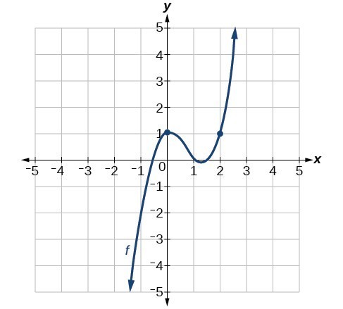
From the graph of the function [latex]y=f\left(x\right)[/latex], estimate each of the following:
To find the functional value, [latex]f\left(a\right)[/latex], find the y-coordinate at [latex]x=a[/latex].
To find the derivative at [latex]x=a[/latex], [latex]\begin{align}{f}^{\prime }\left(a\right)\end{align}[/latex], draw a tangent line at [latex]x=a[/latex], and estimate the slope of that tangent line.
[latex]f\left(0\right)[/latex] is the y-coordinate at [latex]x=0[/latex]. The point has coordinates [latex]\left(0,1\right)[/latex], thus [latex]f\left(0\right)=1[/latex].
[latex]f\left(2\right)[/latex] is the y-coordinate at [latex]x=2[/latex]. The point has coordinates [latex]\left(2,1\right)[/latex], thus [latex]f\left(2\right)=1[/latex].
[latex]\begin{align}{f}^{\prime }\left(0\right)\end{align}[/latex] is found by estimating the slope of the tangent line to the curve at [latex]x=0[/latex]. The tangent line to the curve at [latex]x=0[/latex] appears horizontal. Horizontal lines have a slope of 0, thus [latex]{f}^{\prime }\left(0\right)=0[/latex].
[latex]\begin{align}{f}^{\prime }\left(2\right)\end{align}[/latex] is found by estimating the slope of the tangent line to the curve at [latex]x=2[/latex]. Observe the path of the tangent line to the curve at [latex]x=2[/latex]. As the [latex]x[/latex] value moves one unit to the right, the [latex]y[/latex] value moves up four units to another point on the line. Thus, the slope is 4, so [latex]\begin{align}{f}^{\prime }\left(2\right)\end{align}=4[/latex].
Using the graph of the function [latex]f\left(x\right)={x}^{3}-3x[/latex], estimate: [latex]f\left(1\right)[/latex], [latex]\begin{align}{f}^{\prime }\left(1\right)\end{align}[/latex], [latex]f\left(0\right)[/latex], and [latex]\begin{align}{f}^{\prime }\left(0\right)\end{align}[/latex].

![Graph of the function f(x) = x^3-3x with a viewing window of [-4. 4] by [-5, 7](https://s3-us-west-2.amazonaws.com/courses-images/wp-content/uploads/sites/3675/2018/09/27185408/CNX_Precalc_Figure_12_04_0072.jpg)