When the square root of a number is squared, the result is the original number. Since [latex]{4}^{2}=16[/latex], the square root of [latex]16[/latex] is [latex]4[/latex]. The square root function is the inverse of the squaring function just as subtraction is the inverse of addition. To undo squaring, we take the square root.
square root
The square root of a number [latex]a[/latex] refers to any number [latex]x[/latex] such that [latex]x^2 = a[/latex].
For positive number [latex]a[/latex], there are always two square roots: one positive and one negative.
For example, both [latex]+4[/latex] and [latex]-4[/latex] are square roots of [latex]16[/latex] because both square to give [latex]16[/latex].That is, [latex](+4)^2 = 16[/latex] and [latex](-4)^2 = 16[/latex].
When we talk about square roots in math, we usually mean both the positive and negative numbers that, when multiplied by themselves, give us the original number. In math classes, especially when you’re solving problems or learning algebra, it’s important to think about both these answers unless we’re told to find just one. This helps us understand all the possible solutions to an equation, which is a big part of learning how to solve math problems correctly.
As we explore square roots further, there’s a special version we often use called the principal square root. This refers specifically to the positive square root of a number. It’s helpful to know about this because it’s commonly used in many situations.
principal square root
The principal square root of [latex]a[/latex] is the nonnegative number that when multiplied by itself equals [latex]a[/latex].
The principal square root of [latex]a[/latex] is written as [latex]\sqrt{a}[/latex]. The symbol is called a radical, the term under the symbol is called the radicand, and the entire expression is called a radical expression.
Items of the square root
The square root obtained using a calculator is the principal square root.
Evaluate [latex]\sqrt{25}[/latex].
To evaluate [latex]\sqrt{25}[/latex], you are looking for the principal square root of [latex]25[/latex], which is the positive number that, when squared (multiplied by itself), equals [latex]25[/latex].To find this:
Identify a number that when multiplied by itself gives [latex]25[/latex].
Since [latex]5 \cdot 5 = 25[/latex], and also [latex]-5 \cdot -5 = 25[/latex], there are two square roots: [latex]+5[/latex] and [latex]-5[/latex].
However, we are referring to the principal square root, which is the positive value, when we are finding [latex]\sqrt{25}[/latex].
Thus, [latex]\sqrt{25} = 5[/latex].
The radical symbol of a number implies only a nonnegative root, the principal square root.Evaluate each expression.
[latex]\sqrt{100}[/latex]
[latex]\sqrt{\sqrt{16}}[/latex]
[latex]\sqrt{25+144}[/latex]
[latex]\sqrt{49}-\sqrt{81}[/latex]
[latex]\sqrt{100}=10[/latex] because [latex]{10}^{2}=100[/latex]
[latex]\sqrt{\sqrt{16}}=\sqrt{4}=2[/latex] because [latex]{4}^{2}=16[/latex] and [latex]{2}^{2}=4[/latex]
[latex]\sqrt{25+144}=\sqrt{169}=13[/latex] because [latex]{13}^{2}=169[/latex]
[latex]\sqrt{49}-\sqrt{81}=7 - 9=-2[/latex] because [latex]{7}^{2}=49[/latex] and [latex]{9}^{2}=81[/latex]
Question! For [latex]\sqrt{25+144}[/latex], can we find the square roots before adding?
No!! If we take the square root of each number first: [latex]\sqrt{25}+\sqrt{144}=5+12=17[/latex]. This is not equivalent to [latex]\sqrt{25+144}=13[/latex]. The order of operations requires us to add the terms in the radicand before finding the square root.
Simplifying Square Roots and Expressing Them in Lowest Terms
To simplify a square root means that we rewrite the square root as a rational number times the square root of a number that has no perfect square factors. The act of changing a square root into such a form is simplifying the square root. Before discussing how to simplify a square root, we need to introduce a rule about square roots.
the product rule for square roots
The square root of a product of numbers equals the product of the square roots of those number.
Given that [latex]a[/latex] and [latex]b[/latex] are nonnegative real numbers,
Using this formula, we can factor an integer inside a square root into a perfect square times another integer. Then the square root can be applied to the perfect square, leaving an integer times the square root of another integer. If the number remaining under the square root has no perfect square factors, then we’ve simplified the irrational number into lowest terms.
A perfect square is an integer that can be expressed as the square of another integer. For example, [latex]16[/latex], [latex]25[/latex], and [latex]36[/latex] are perfect squares because they are [latex]4^2[/latex], [latex]5^2[/latex], and [latex]6^2[/latex], respectively.How to: Simplify square roots into lowest terms when [latex]n[/latex] is an integer
Step 1: Determine the largest perfect square factor of [latex]n[/latex], which we denote [latex]a^2[/latex].
Step 2: Factor [latex]n[/latex] into [latex]a^2×b[/latex].
Step 4: Write [latex]\sqrt{n}[/latex] in its simplified form, [latex]a\sqrt{b}[/latex].
To simplify the given radical expressions, we’ll break down the numbers into their prime factors and simplify the radicals accordingly, while also considering the powers of the variables. Here are the steps:First, factor [latex]300[/latex] into its prime factors:
[latex]300 = 2^2 \cdot 3 \cdot 5^2[/latex]
Now, extract the square roots of the perfect squares:
[latex]\begin{align} \sqrt{300} &= \sqrt{2^2 \cdot 3 \cdot 5^2} && \text{Factor the number into prime factors.} \\ &= \sqrt{2^2} \cdot \sqrt{3} \cdot \sqrt{5^2} && \text{Separate each factor under its own square root.} \\ &= 2 \cdot \sqrt{3} \cdot 5 && \text{Simplify the square roots of perfect squares.} \\ &= 10\sqrt{3} && \text{Multiply the results to get the simplified form.} \end{align}[/latex]
Simplify [latex]\sqrt{162{a}^{5}{b}^{4}}[/latex].
\begin{align} \sqrt{162a^5b^4} &= \sqrt{2 \cdot 3^4 \cdot a^5 \cdot b^4} && \text{Factor the number into prime factors and express variables.} \\ &= \sqrt{2 \cdot (3^2)^2 \cdot a^4 \cdot a \cdot (b^2)^2} && \text{Break down the expression to show squares for clarity.} \\ &= \sqrt{2} \cdot \sqrt{(3^2)^2} \cdot \sqrt{a^4} \cdot \sqrt{a} \cdot \sqrt{(b^2)^2} && \text{Separate each factor under its own square root.} \\ &= \sqrt{2} \cdot 3^2 \cdot a^2 \cdot \sqrt{a} \cdot b^2 && \text{Simplify the square roots of perfect squares.} \\ &= 9a^2b^2 \cdot \sqrt{2a} && \text{Combine the constants and simplify further to finalize.} \end{align}
For the variable [latex]x[/latex], [latex]\sqrt{x^2} = |x|[/latex] , but why is that?When you square any values, the result is always non-negative, meaning it’s either positive or zero. Then, when you take the square root of this non-negative squared value, you get back the original number without its sign—just its size or magnitude. Thus, taking the square root of [latex]x^2[/latex] always yields the absolute value of [latex]x[/latex] ensuring that we consider [latex]x[/latex] in its non-negative form.
definition
Identifying Horizontal Shifts
We just saw that the vertical shift is a change to the output, or outside, of the function. We will now look at how changes to input, on the inside of the function, change its graph and meaning. A shift to the input results in a movement of the graph of the function left or right in what is known as a horizontal shift.
horizontal shift
A horizontal shift occurs when you add or subtract a constant value to the input [latex]x[/latex] of the function [latex]f(x)[/latex].
This shifts the graph of the function horizontally.
Rightward shift: If you subtract a constant [latex]c[/latex] from [latex]x[/latex] before applying the function [latex]f[/latex], the graph of the function shifts to the right by [latex]c[/latex] units.
[latex]g(x) = f(x-c)[/latex]
Leftward shift: If you add a constant [latex]c[/latex] to [latex]x[/latex] before applying the function [latex]f[/latex], the graph of the function shifts to the left by [latex]c[/latex] units.
[latex]h(x) = f(x+c)[/latex]
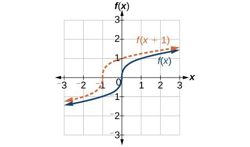
The image shows the graph of the cube root function [latex]f(x) = \sqrt[3]{x}[/latex] (solid blue line) and its horizontally shifted version [latex]f(x + 1)[/latex] (dashed orange line).Original Function [latex]f(x)[/latex]
The solid blue curve represents the original function [latex]\sqrt[3]{x}[/latex].
The function [latex]f(x)[/latex] passes through the origin [latex](0,0)[/latex] because [latex]\sqrt[3]{0} = 0[/latex].
Horizontally Shifted Function [latex]f(x+1)[/latex]
The dashed orange curve represents the function [latex]f(x+1) = \sqrt[3]{x+1}[/latex].
Each point on the graph of [latex]f(x+1)[/latex] is exactly [latex]1[/latex] unit to the left of the corresponding point on the graph of [latex]f(x)[/latex].
For example:
If [latex]x=0[/latex], then [latex]\sqrt[3]{0+1} = \sqrt[3]{1} = 1[/latex].
If [latex]x=-2[/latex], then [latex]\sqrt[3]{-2+1} = \sqrt[3]{-1} = -1[/latex].
A horizontal shift involves moving the graph of a function left or right without altering its shape. In this case, adding [latex]1[/latex] to the input of the function [latex]f(x) = \sqrt[3]{x}[/latex] results in a horizontal shift of the graph to the left by [latex]1[/latex] unit.
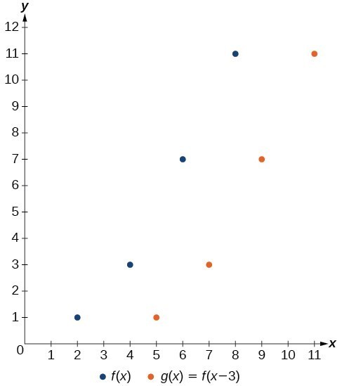
A function [latex]f\left(x\right)[/latex] is given below. Create a table for the function [latex]g\left(x\right)=f\left(x - 3\right)[/latex].
[latex]x[/latex]
2
4
6
8
[latex]f\left(x\right)[/latex]
1
3
7
11
The formula [latex]g\left(x\right)=f\left(x - 3\right)[/latex] tells us that the output values of [latex]g[/latex] are the same as the output value of [latex]f[/latex] when the input value is 3 less than the original value. For example, we know that [latex]f\left(2\right)=1[/latex]. To get the same output from the function [latex]g[/latex], we will need an input value that is 3 larger. We input a value that is 3 larger for [latex]g\left(x\right)[/latex] because the function takes 3 away before evaluating the function [latex]f[/latex].
We continue with the other values to create this table.
[latex]x[/latex]
5
7
9
11
[latex]x - 3[/latex]
2
4
6
8
[latex]f\left(x\right)[/latex]
1
3
7
11
[latex]g\left(x\right)[/latex]
1
3
7
11
The result is that the function [latex]f\left(x\right)[/latex] has been shifted to the right by 3. Notice the output values for [latex]g\left(x\right)[/latex] remain the same as the output values for [latex]f\left(x\right)[/latex], but the corresponding input values, [latex]x[/latex], have shifted to the right by 3. Specifically, 2 shifted to 5, 4 shifted to 7, 6 shifted to 9, and 8 shifted to 11.
Analysis of the Solution
The graph below represents both of the functions. We can see the horizontal shift in each point.
The function [latex]G\left(m\right)[/latex] gives the number of gallons of gas required to drive [latex]m[/latex] miles. Interpret [latex]G\left(m\right)+10[/latex] and [latex]G\left(m+10\right)[/latex].
[latex]G\left(m\right)+10[/latex] can be interpreted as adding [latex]10[/latex] to the output, gallons. This is the gas required to drive [latex]m[/latex] miles, plus another [latex]10[/latex] gallons of gas. The graph would indicate a vertical shift.[latex]G\left(m+10\right)[/latex] can be interpreted as adding [latex]10[/latex]to the input, miles. So this is the number of gallons of gas required to drive [latex]10[/latex] miles more than [latex]m[/latex] miles. The graph would indicate a horizontal shift.
How To: Given a tabular function, create a new row to represent a horizontal shift.
Identify the input row or column.
Determine the magnitude of the shift.
Add the shift to the value in each input cell.
A function [latex]f\left(x\right)[/latex] is given below. Create a table for the function [latex]g\left(x\right)=f\left(x - 3\right)[/latex].
[latex]x[/latex]
2
4
6
8
[latex]f\left(x\right)[/latex]
1
3
7
11
The formula [latex]g\left(x\right)=f\left(x - 3\right)[/latex] tells us that the output values of [latex]g[/latex] are the same as the output value of [latex]f[/latex] when the input value is 3 less than the original value. For example, we know that [latex]f\left(2\right)=1[/latex]. To get the same output from the function [latex]g[/latex], we will need an input value that is 3 larger. We input a value that is 3 larger for [latex]g\left(x\right)[/latex] because the function takes 3 away before evaluating the function [latex]f[/latex].
We continue with the other values to create this table.
[latex]x[/latex]
5
7
9
11
[latex]x - 3[/latex]
2
4
6
8
[latex]f\left(x\right)[/latex]
1
3
7
11
[latex]g\left(x\right)[/latex]
1
3
7
11
The result is that the function [latex]g\left(x\right)[/latex] has been shifted to the right by 3. Notice the output values for [latex]g\left(x\right)[/latex] remain the same as the output values for [latex]f\left(x\right)[/latex], but the corresponding input values, [latex]x[/latex], have shifted to the right by 3. Specifically, 2 shifted to 5, 4 shifted to 7, 6 shifted to 9, and 8 shifted to 11.
Analysis of the Solution
The graph represents both of the functions. We can see the horizontal shift in each point.
transformed functions
The formula for a transformed function is [latex]g(x) = \pm a \cdot f\big(\pm b(x - h)\big) + k[/latex] where:
[latex]\pm a[/latex] describes the vertical reflection and stretch/compression
[latex]\pm b[/latex] describes the horizontal reflection and stretch/compression
[latex]h[/latex] describes the horizontal shift, and
[latex]k[/latex] describes the vertical shift
Find the parent function. If it's not given to you, check the toolkit functions.
Identify any shifts.
Identify any reflections, stretches or compresses.
Write the function using [latex]g(x) = a \cdot f\big(b(x - h)\big) + k[/latex]
Writing Functions Given the Transformed Graph
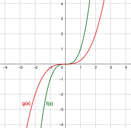
The graph shows two function: The toolkit function [latex]f(x) = x^3[/latex] (green) and [latex]g(x)[/latex] (red). Relate this new function [latex]g\left(x\right)[/latex] to [latex]f\left(x\right)[/latex], and then find a formula for [latex]g\left(x\right)[/latex].
The red curve [latex]g(x)[/latex] appears to be less steep compared to the green curve [latex]f(x)[/latex]. This suggests a vertical compression.If [latex]g(x)[/latex] is a vertical compression of [latex]f(x)[/latex], we have: [latex]g(x) = a \cdot f(x)[/latex], where [latex]0 < a < 1[/latex].To determine [latex]a[/latex], it is helpful to look for a point on the graph that is relatively clear.
In this graph, it appears that [latex]g\left(2\right)=2[/latex].
With the basic cubic function at the same input, [latex]f\left(2\right)={2}^{3}=8[/latex].
Based on that, it appears that the outputs of [latex]g[/latex] are [latex]\frac{1}{4}[/latex] the outputs of the function [latex]f[/latex] because [latex]2=\frac{1}{4} \cdot 8[/latex].
Relate the function [latex]g\left(x\right)[/latex] to [latex]f\left(x\right)[/latex].
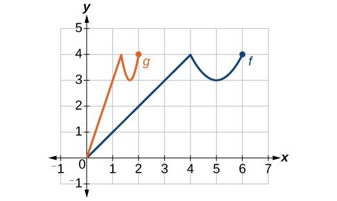
The orange graph [latex]g(x)[/latex] appears to be a horizontally compressed version of the blue graph of [latex]f(x)[/latex].
[latex]\\[/latex]
If [latex]g(x)[/latex] is a horizontal compression of [latex]f(x)[/latex], we have: [latex]g(x) = f(b \cdot x)[/latex], where [latex]b > 1[/latex]. The graph is compressed by [latex]\dfrac{1}{b}[/latex].To determine [latex]b[/latex], it is helpful to look for a point on the graph that is relatively clear.
In the compressed graph [latex]g(x)[/latex], the end point is [latex](2, 4)[/latex].
The end point of [latex]f(x)[/latex] is [latex](6,4)[/latex].
We can see that the [latex]x[/latex]-values have been compressed by [latex]\frac{1}{3}[/latex], because [latex]2=\frac{1}{3} \cdot 6[/latex].
This means that [latex]\dfrac{1}{b} = \dfrac{1}{3}[/latex], which means [latex]b = 3[/latex].
Thus, [latex]g(x)=f(3x)[/latex].
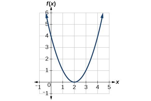
The graph below represents a transformation of the toolkit function [latex]f\left(x\right)={x}^{2}[/latex]. Relate this new function [latex]g\left(x\right)[/latex] to [latex]f\left(x\right)[/latex], and then find a formula for [latex]g\left(x\right)[/latex].
Notice that the graph is identical in shape to the [latex]f\left(x\right)={x}^{2}[/latex] function, but the [latex]x[/latex]-values are shifted to the right 2 units. The vertex used to be at (0,0), but now the vertex is at (2,0). The graph is the basic quadratic function shifted 2 units to the right, so
Notice how we must input the value [latex]x=2[/latex] to get the output value [latex]y=0[/latex]; the [latex]x[/latex]-values must be 2 units larger because of the shift to the right by 2 units. We can then use the definition of the [latex]f\left(x\right)[/latex] function to write a formula for [latex]g\left(x\right)[/latex] by evaluating [latex]f\left(x - 2\right)[/latex].
To determine whether the shift is [latex]+2[/latex] or [latex]-2[/latex] , consider a single reference point on the graph. For a quadratic, looking at the vertex point is convenient. In the original function, [latex]f\left(0\right)=0[/latex]. In our shifted function, [latex]g\left(2\right)=0[/latex]. To obtain the output value of 0 from the function [latex]f[/latex], we need to decide whether a plus or a minus sign will work to satisfy [latex]g\left(2\right)=f\left(x - 2\right)=f\left(0\right)=0[/latex]. For this to work, we will need to subtract 2 units from our input values.
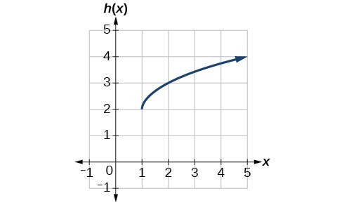
Write a formula for the graph shown, which is a transformation of the toolkit square root function.
The graph of the toolkit function starts at the origin, so this graph has been shifted 1 to the right and up 2. In function notation, we could write that as
Using the formula for the square root function, we can write
[latex]h\left(x\right)=\sqrt{x - 1}+2[/latex]
Analysis of the Solution
Note that this transformation has changed the domain and range of the function. This new graph has domain [latex]\left[1,\infty \right)[/latex] and range [latex]\left[2,\infty \right)[/latex].
Writing Functions Given the Transformed Graph
Graph functions using a single transformation.
Graph functions using a combination of transformations.
Determine whether a function is even, odd, or neither from its graph.
Describe transformations based on a function formula.
Give the formula of a function based on its transformations.
Figure 1. (credit: "Misko"/Flickr)
We all know that a flat mirror enables us to see an accurate image of ourselves and whatever is behind us. When we tilt the mirror, the images we see may shift horizontally or vertically. But what happens when we bend a flexible mirror? Like a carnival funhouse mirror, it presents us with a distorted image of ourselves, stretched or compressed horizontally or vertically. In a similar way, we can distort or transform mathematical functions to better adapt them to describing objects or processes in the real world. In this section, we will take a look at several kinds of transformations.
Graphing Functions Using Reflections about the Axes
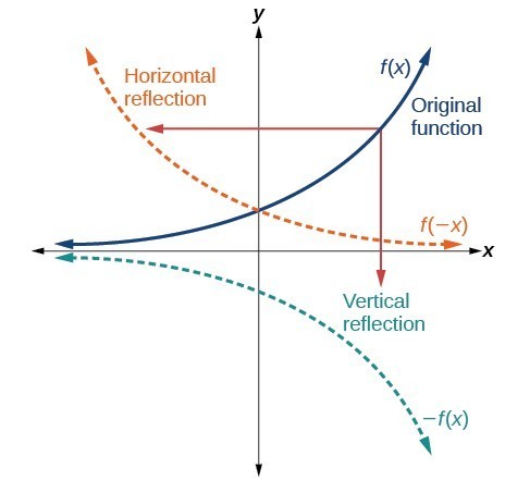
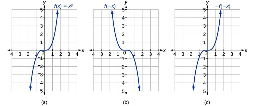
Another transformation that can be applied to a function is a reflection over the [latex]x[/latex]- or [latex]y[/latex]-axis. A vertical reflection reflects a graph vertically across the [latex]x[/latex]-axis, while a horizontal reflection reflects a graph horizontally across the [latex]y[/latex]-axis.
Notice that the vertical reflection produces a new graph that is a mirror image of the base or original graph about the [latex]x[/latex]-axis. The horizontal reflection produces a new graph that is a mirror image of the base or original graph about the [latex]y[/latex]-axis.
reflections
A vertical reflectionreflects a graph vertically across the [latex]x[/latex]-axis. This transformation changes the sign of the output values of [latex]f(x)[/latex].
If you reflect the graph of a function [latex]f(x)[/latex] over the [latex]x[/latex]-axis, the new function [latex]g(x)[/latex] is given by:
[latex]g(x) = -f(x)[/latex]
A horizontal reflectionreflects a graph horizontally across the [latex]y[/latex]-axis. This transformation changes the sign of the input values of [latex]f(x)[/latex].
If you reflect the graph of a function [latex]f(x)[/latex] over the [latex]y[/latex]-axis, the new function [latex]g(x)[/latex] is given by:
[latex]g(x) = f(-x)[/latex]
How To: Given a function, reflect the graph both vertically and horizontally.
Multiply all outputs by –1 for a vertical reflection. The new graph is a reflection of the original graph about the [latex]x[/latex]-axis.
Multiply all inputs by –1 for a horizontal reflection. The new graph is a reflection of the original graph about the [latex]y[/latex]-axis.
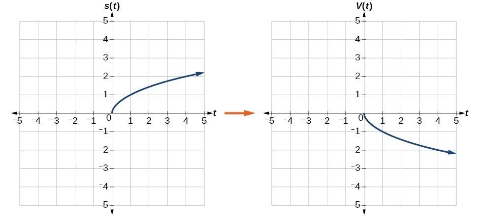
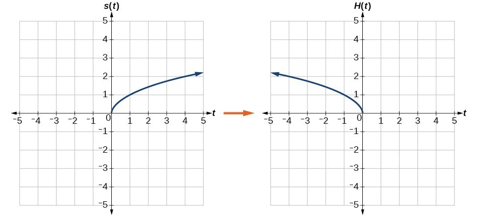
Reflect the graph of [latex]s\left(t\right)=\sqrt{t}[/latex]
vertically
horizontally
Reflecting the graph vertically means that each output value will be reflected over the horizontal [latex]t[/latex]-axis as shown below. Vertical reflection of the square root function
Table of values
[latex]t[/latex]
[latex]s(t) = \sqrt{t}[/latex]
Reflected Function [latex]V(t)[/latex]
[latex]0[/latex]
[latex]0[/latex]
[latex]0[/latex]
[latex]1[/latex]
[latex]1[/latex]
[latex]-1[/latex]
[latex]4[/latex]
[latex]2[/latex]
[latex]-2[/latex]
Because each output value is the opposite of the original output value, we can write
[latex]V\left(t\right)=-s\left(t\right)\text{ or }V\left(t\right)=-\sqrt{t}[/latex]
Notice that this is an outside change, or vertical shift, that affects the output [latex]s\left(t\right)[/latex] values, so the negative sign belongs outside of the function.
Reflecting horizontally means that each input value will be reflected over the vertical axis as shown below. Horizontal reflection of the square root function
Table for [latex]s(t) = \sqrt{t}[/latex]
[latex]t[/latex]
[latex]0[/latex]
[latex]1[/latex]
[latex]4[/latex]
[latex]s(t) = \sqrt{t}[/latex]
[latex]0[/latex]
[latex]1[/latex]
[latex]2[/latex]
Table for reflected function
[latex]t[/latex]
[latex]0[/latex]
[latex]-1[/latex]
[latex]-4[/latex]
[latex]H(t)[/latex]
[latex]0[/latex]
[latex]1[/latex]
[latex]2[/latex]
Because each input value is the opposite of the original input value, we can write
[latex]H\left(t\right)=s\left(-t\right)\text{ or }H\left(t\right)=\sqrt{-t}[/latex]
Notice that this is an inside change or horizontal change that affects the input values, so the negative sign is on the inside of the function.
Note that these transformations can affect the domain and range of the functions. While the original square root function has domain [latex]\left[0,\infty \right)[/latex] and range [latex]\left[0,\infty \right)[/latex], the vertical reflection gives the [latex]V\left(t\right)[/latex] function the range [latex]\left(-\infty ,0\right][/latex] and the horizontal reflection gives the [latex]H\left(t\right)[/latex] function the domain [latex]\left(-\infty ,0\right][/latex].
A function [latex]f\left(x\right)[/latex] is given. Create a table for the functions below.
[latex]g\left(x\right)=-f\left(x\right)[/latex]
[latex]h\left(x\right)=f\left(-x\right)[/latex]
[latex]x[/latex]
[latex]2[/latex]
[latex]4[/latex]
[latex]6[/latex]
[latex]8[/latex]
[latex]f\left(x\right)[/latex]
[latex]1[/latex]
[latex]3[/latex]
[latex]7[/latex]
[latex]11[/latex]
For [latex]g\left(x\right)[/latex], the negative sign outside the function indicates a vertical reflection, so the [latex]x[/latex]-values stay the same and each output value will be the opposite of the original output value.
[latex]x[/latex]
[latex]2[/latex]
[latex]4[/latex]
[latex]6[/latex]
[latex]8[/latex]
[latex]g\left(x\right)[/latex]
[latex]–1[/latex]
[latex]–3[/latex]
[latex]–7[/latex]
[latex]–11[/latex]
For [latex]h\left(x\right)[/latex], the negative sign inside the function indicates a horizontal reflection, so each input value will be the opposite of the original input value and the [latex]h\left(x\right)[/latex] values stay the same as the [latex]f\left(x\right)[/latex] values.
[latex]x[/latex]
[latex]−2[/latex]
[latex]−4[/latex]
[latex]−6[/latex]
[latex]−8[/latex]
[latex]h\left(x\right)[/latex]
[latex]1[/latex]
[latex]3[/latex]
[latex]7[/latex]
[latex]11[/latex]
A function [latex]f\left(x\right)[/latex] is given. Create a table for the functions below.
[latex]g\left(x\right)=-f\left(x\right)[/latex]
[latex]h\left(x\right)=f\left(-x\right)[/latex]
[latex]x[/latex]
2
4
6
8
[latex]f\left(x\right)[/latex]
1
3
7
11
For [latex]g\left(x\right)[/latex], the negative sign outside the function indicates a vertical reflection, so the x-values stay the same and each output value will be the opposite of the original output value.
[latex]x[/latex]
2
4
6
8
[latex]g\left(x\right)[/latex]
–1
–3
–7
–11
For [latex]h\left(x\right)[/latex], the negative sign inside the function indicates a horizontal reflection, so each input value will be the opposite of the original input value and the [latex]h\left(x\right)[/latex] values stay the same as the [latex]f\left(x\right)[/latex] values.
[latex]x[/latex]
−2
−4
−6
−8
[latex]h\left(x\right)[/latex]
1
3
7
11
[latex]x[/latex]
−2
0
2
4
[latex]f\left(x\right)[/latex]
5
10
15
20
Using the function [latex]f\left(x\right)[/latex] given in the table above, create a table for the functions below.
a. [latex]g\left(x\right)=-f\left(x\right)[/latex]
b. [latex]h\left(x\right)=f\left(-x\right)[/latex]
[latex]g\left(x\right)=-f\left(x\right)[/latex]
[latex]x[/latex]
-2
0
2
4
[latex]g\left(x\right)[/latex]
[latex]-5[/latex]
[latex]-10[/latex]
[latex]-15[/latex]
[latex]-20[/latex]
[latex]h\left(x\right)=f\left(-x\right)[/latex]
[latex]x[/latex]
-2
0
2
4
[latex]h\left(x\right)[/latex]
15
10
5
unknown
Determining Even and Odd Functions
Some functions have symmetry, meaning their graphs remain unchanged when reflected. For example, reflecting the toolkit functions [latex]f(x) = x^2[/latex] or [latex]f(x) = |x|[/latex] horizontally across the y-axis will produce the same graph. We call these functions even functions because they are symmetric about the y-axis.
If the graph of [latex]f(x) = x^3[/latex] or [latex]f(x) = \dfrac{1}{x}[/latex] is reflected across both the x-axis and y-axis, the result is also the original graph.
These graphs are symmetric about the origin, and we call functions with this type of symmetry odd functions.
A function can be neither even nor odd if it does not exhibit either symmetry. For example, [latex]f\left(x\right)={2}^{x}[/latex] is neither even nor odd. Also, the only function that is both even and odd is the constant function [latex]f\left(x\right)=0[/latex].
even and odd functions
A function is called an even function if for every input [latex]x[/latex]
[latex]f\left(x\right)=f\left(-x\right)[/latex]
The graph of an even function is symmetric about the [latex]y\text{-}[/latex] axis.
A function is called an odd function if for every input [latex]x[/latex]
[latex]f\left(x\right)=-f\left(-x\right)[/latex]
The graph of an odd function is symmetric about the origin.
How To: Given the formula for a function, determine if the function is even, odd, or neither.
Determine whether the function satisfies [latex]f\left(x\right)=f\left(-x\right)[/latex]. If it does, it is even.
Determine whether the function satisfies [latex]f\left(x\right)=-f\left(-x\right)[/latex]. If it does, it is odd.
If the function does not satisfy either rule, it is neither even nor odd.
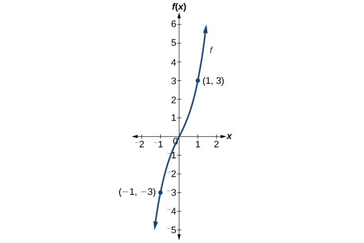
Is the function [latex]f\left(x\right)={x}^{3}+2x[/latex] even, odd, or neither?
Without looking at a graph, we can determine whether the function is even or odd by finding formulas for the reflections and determining if they return us to the original function. Let’s begin with the rule for even functions.
Because [latex]-f\left(-x\right)=f\left(x\right)[/latex], this is an odd function.
Analysis of the Solution
Consider the graph of [latex]f[/latex]. Notice that the graph is symmetric about the origin. For every point [latex]\left(x,y\right)[/latex] on the graph, the corresponding point [latex]\left(-x,-y\right)[/latex] is also on the graph. For example, (1, 3) is on the graph of [latex]f[/latex], and the corresponding point [latex]\left(-1,-3\right)[/latex] is also on the graph.
Key Equations
Vertical shift
[latex]g\left(x\right)=f\left(x\right)+k[/latex] (up for [latex]k>0[/latex] )
Horizontal shift
[latex]g\left(x\right)=f\left(x-h\right)[/latex] (right for [latex]h>0[/latex] )
A function can be shifted vertically by adding a constant to the output.
A function can be shifted horizontally by adding a constant to the input.
Relating the shift to the context of a problem makes it possible to compare and interpret vertical and horizontal shifts.
Vertical and horizontal shifts are often combined.
A vertical reflection reflects a graph about the [latex]x\text{-}[/latex] axis. A graph can be reflected vertically by multiplying the output by –1.
A horizontal reflection reflects a graph about the [latex]y\text{-}[/latex] axis. A graph can be reflected horizontally by multiplying the input by –1.
A graph can be reflected both vertically and horizontally. The order in which the reflections are applied does not affect the final graph.
A function presented in tabular form can also be reflected by multiplying the values in the input and output rows or columns accordingly.
A function presented as an equation can be reflected by applying transformations one at a time.
Even functions are symmetric about the [latex]y\text{-}[/latex] axis, whereas odd functions are symmetric about the origin.
Even functions satisfy the condition [latex]f\left(x\right)=f\left(-x\right)[/latex].
Odd functions satisfy the condition [latex]f\left(x\right)=-f\left(-x\right)[/latex].
A function can be odd, even, or neither.
A function can be compressed or stretched vertically by multiplying the output by a constant.
A function can be compressed or stretched horizontally by multiplying the input by a constant.
The order in which different transformations are applied does affect the final function. Both vertical and horizontal transformations must be applied in the order given. However, a vertical transformation may be combined with a horizontal transformation in any order.
Glossary
even function
a function whose graph is unchanged by horizontal reflection, [latex]f\left(x\right)=f\left(-x\right)[/latex], and is symmetric about the [latex]y\text{-}[/latex] axis
horizontal compression
a transformation that compresses a function’s graph horizontally, by multiplying the input by a constant [latex]b>1[/latex]
horizontal reflection
a transformation that reflects a function’s graph across the y-axis by multiplying the input by [latex]-1[/latex]
horizontal shift
a transformation that shifts a function’s graph left or right by adding a positive or negative constant to the input
horizontal stretch
a transformation that stretches a function’s graph horizontally by multiplying the input by a constant [latex]0
odd function
a function whose graph is unchanged by combined horizontal and vertical reflection, [latex]f\left(x\right)=-f\left(-x\right)[/latex], and is symmetric about the origin
vertical compression
a function transformation that compresses the function’s graph vertically by multiplying the output by a constant [latex]0
vertical reflection
a transformation that reflects a function’s graph across the x-axis by multiplying the output by [latex]-1[/latex]
vertical shift
a transformation that shifts a function’s graph up or down by adding a positive or negative constant to the output
vertical stretch
a transformation that stretches a function’s graph vertically by multiplying the output by a constant [latex]a>1[/latex]
transformed functions
The formula for a transformed function is [latex]g(x) = \pm a \cdot f\big(\pm b(x - h)\big) + k[/latex] where:
[latex]\pm a[/latex] describes the vertical reflection and stretch/compression
[latex]\pm b[/latex] describes the horizontal reflection and stretch/compression
[latex]h[/latex] describes the horizontal shift, and
[latex]k[/latex] describes the vertical shift
Find the parent function. If it's not given to you, check the toolkit functions.
Identify any shifts.
Identify any reflections, stretches or compresses.
Write the function using [latex]g(x) = a \cdot f\big(b(x - h)\big) + k[/latex]
Writing Functions Given the Transformed Graph
The graph shows two function: The toolkit function [latex]f(x) = x^3[/latex] (green) and [latex]g(x)[/latex] (red). Relate this new function [latex]g\left(x\right)[/latex] to [latex]f\left(x\right)[/latex], and then find a formula for [latex]g\left(x\right)[/latex].
The red curve [latex]g(x)[/latex] appears to be less steep compared to the green curve [latex]f(x)[/latex]. This suggests a vertical compression.If [latex]g(x)[/latex] is a vertical compression of [latex]f(x)[/latex], we have: [latex]g(x) = a \cdot f(x)[/latex], where [latex]0 < a < 1[/latex].To determine [latex]a[/latex], it is helpful to look for a point on the graph that is relatively clear.
In this graph, it appears that [latex]g\left(2\right)=2[/latex].
With the basic cubic function at the same input, [latex]f\left(2\right)={2}^{3}=8[/latex].
Based on that, it appears that the outputs of [latex]g[/latex] are [latex]\frac{1}{4}[/latex] the outputs of the function [latex]f[/latex] because [latex]2=\frac{1}{4} \cdot 8[/latex].
Relate the function [latex]g\left(x\right)[/latex] to [latex]f\left(x\right)[/latex].
The orange graph [latex]g(x)[/latex] appears to be a horizontally compressed version of the blue graph of [latex]f(x)[/latex].
[latex]\\[/latex]
If [latex]g(x)[/latex] is a horizontal compression of [latex]f(x)[/latex], we have: [latex]g(x) = f(b \cdot x)[/latex], where [latex]b > 1[/latex]. The graph is compressed by [latex]\dfrac{1}{b}[/latex].To determine [latex]b[/latex], it is helpful to look for a point on the graph that is relatively clear.
In the compressed graph [latex]g(x)[/latex], the end point is [latex](2, 4)[/latex].
The end point of [latex]f(x)[/latex] is [latex](6,4)[/latex].
We can see that the [latex]x[/latex]-values have been compressed by [latex]\frac{1}{3}[/latex], because [latex]2=\frac{1}{3} \cdot 6[/latex].
This means that [latex]\dfrac{1}{b} = \dfrac{1}{3}[/latex], which means [latex]b = 3[/latex].
Thus, [latex]g(x)=f(3x)[/latex].
The graph below represents a transformation of the toolkit function [latex]f\left(x\right)={x}^{2}[/latex]. Relate this new function [latex]g\left(x\right)[/latex] to [latex]f\left(x\right)[/latex], and then find a formula for [latex]g\left(x\right)[/latex].
Notice that the graph is identical in shape to the [latex]f\left(x\right)={x}^{2}[/latex] function, but the [latex]x[/latex]-values are shifted to the right 2 units. The vertex used to be at (0,0), but now the vertex is at (2,0). The graph is the basic quadratic function shifted 2 units to the right, so
Notice how we must input the value [latex]x=2[/latex] to get the output value [latex]y=0[/latex]; the [latex]x[/latex]-values must be 2 units larger because of the shift to the right by 2 units. We can then use the definition of the [latex]f\left(x\right)[/latex] function to write a formula for [latex]g\left(x\right)[/latex] by evaluating [latex]f\left(x - 2\right)[/latex].
To determine whether the shift is [latex]+2[/latex] or [latex]-2[/latex] , consider a single reference point on the graph. For a quadratic, looking at the vertex point is convenient. In the original function, [latex]f\left(0\right)=0[/latex]. In our shifted function, [latex]g\left(2\right)=0[/latex]. To obtain the output value of 0 from the function [latex]f[/latex], we need to decide whether a plus or a minus sign will work to satisfy [latex]g\left(2\right)=f\left(x - 2\right)=f\left(0\right)=0[/latex]. For this to work, we will need to subtract 2 units from our input values.
Write a formula for the graph shown in Figure 24, which is a transformation of the toolkit square root function.
Figure 24
The graph of the toolkit function starts at the origin, so this graph has been shifted 1 to the right and up 2. In function notation, we could write that as
Using the formula for the square root function, we can write
[latex]h\left(x\right)=\sqrt{x - 1}+2[/latex]
Analysis of the Solution
Note that this transformation has changed the domain and range of the function. This new graph has domain [latex]\left[1,\infty \right)[/latex] and range [latex]\left[2,\infty \right)[/latex].
Writing Functions Given the Transformed Graph
Write a formula for a transformation of the toolkit reciprocal function [latex]f\left(x\right)=\frac{1}{x}[/latex] that shifts the function’s graph one unit to the right and one unit up.

 Original Function [latex]f(x)[/latex]

 The graph shows two function: The toolkit function [latex]f(x) = x^3[/latex] (green) and [latex]g(x)[/latex] (red). Relate this new function [latex]g\left(x\right)[/latex] to [latex]f\left(x\right)[/latex], and then find a formula for [latex]g\left(x\right)[/latex].
 Relate the function [latex]g\left(x\right)[/latex] to [latex]f\left(x\right)[/latex].