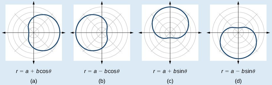
The word limaçon is Old French for “snail,” a name that describes the shape of the graph. As mentioned earlier, the cardioid is a member of the limaçon family, and we can see the similarities in the graphs. The other images in this category include the one-loop limaçon and the two-loop (or inner-loop) limaçon. One-loop limaçons are sometimes referred to as dimpled limaçons when [latex]1<\frac{a}{b}<2[/latex] and convex limaçons when [latex]\frac{a}{b}\ge 2[/latex].
limaçons
The formulas that produce the graph of a dimpled one-loop limaçon are given by [latex]r=a\pm b\cos \theta[/latex] and [latex]r=a\pm b\sin \theta[/latex] where [latex]a>0,b>0,\text{and 1<}\frac{a}{b}<2[/latex]. All four graphs are shown in Figure 9.
How To: Given a polar equation for a one-loop limaçon, sketch the graph.
Test the equation for symmetry. Remember that failing a symmetry test does not mean that the shape will not exhibit symmetry. Often the symmetry may reveal itself when the points are plotted.
Find the zeros.
Find the maximum values according to the trigonometric expression.
Make a table.
Plot the points and sketch the graph.
Graph the equation [latex]r=4 - 3\sin \theta[/latex].
First, testing the equation for symmetry, we find that it fails all three symmetry tests, meaning that the graph may or may not exhibit symmetry, so we cannot use the symmetry to help us graph it. However, this equation has a graph that clearly displays symmetry with respect to the line [latex]\theta =\frac{\pi }{2}[/latex], yet it fails all the three symmetry tests. A graphing calculator will immediately illustrate the graph’s reflective quality.Next, we find the zeros and maximum, and plot the reflecting points to verify any symmetry. Setting [latex]r=0[/latex] results in [latex]\theta[/latex] being undefined. What does this mean? How could [latex]\theta[/latex] be undefined? The angle [latex]\theta[/latex] is undefined for any value of [latex]\sin \theta >1[/latex]. Therefore, [latex]\theta[/latex] is undefined because there is no value of [latex]\theta[/latex] for which [latex]\sin \theta >1[/latex]. Consequently, the graph does not pass through the pole. Perhaps the graph does cross the polar axis, but not at the pole. We can investigate other intercepts by calculating [latex]r[/latex] when [latex]\theta =0[/latex].
So, there is at least one polar axis intercept at [latex]\left(4,0\right)[/latex].
Next, as the maximum value of the sine function is 1 when [latex]\theta =\frac{\pi }{2}[/latex], we will substitute [latex]\theta =\frac{\pi }{2}[/latex] into the equation and solve for [latex]r[/latex]. Thus, [latex]r=1[/latex].
Make a table of the coordinates similar to the table below.
[latex]\theta[/latex]
[latex]0[/latex]
[latex]\frac{\pi }{6}[/latex]
[latex]\frac{\pi }{3}[/latex]
[latex]\frac{\pi }{2}[/latex]
[latex]\frac{2\pi }{3}[/latex]
[latex]\frac{5\pi }{6}[/latex]
[latex]\pi[/latex]
[latex]\frac{7\pi }{6}[/latex]
[latex]\frac{4\pi }{3}[/latex]
[latex]\frac{3\pi }{2}[/latex]
[latex]\frac{5\pi }{3}[/latex]
[latex]\frac{11\pi }{6}[/latex]
[latex]2\pi[/latex]
[latex]r[/latex]
4
2.5
1.4
1
1.4
2.5
4
5.5
6.6
7
6.6
5.5
4
One-loop limaçon
Analysis of the Solution
This is an example of a curve for which making a table of values is critical to producing an accurate graph. The symmetry tests fail; the zero is undefined. While it may be apparent that an equation involving [latex]\sin \theta[/latex] is likely symmetric with respect to the line [latex]\theta =\frac{\pi }{2}[/latex], evaluating more points helps to verify that the graph is correct.
Another type of limaçon, the inner-loop limaçon, is named for the loop formed inside the general limaçon shape. It was discovered by the German artist Albrecht Dürer(1471-1528), who revealed a method for drawing the inner-loop limaçon in his 1525 book Underweysung der Messing. A century later, the father of mathematician Blaise Pascal, Étienne Pascal(1588-1651), rediscovered it.
inner-loop limaçons
The formulas that generate the inner-loop limaçons are given by [latex]r=a\pm b\cos \theta[/latex] and [latex]r=a\pm b\sin \theta[/latex] where [latex]a>0,b>0[/latex], and [latex]a
Sketch the graph of [latex]r=2+5\text{cos}\theta[/latex].
Testing for symmetry, we find that the graph of the equation is symmetric about the polar axis. Next, finding the zeros reveals that when [latex]r=0,\theta =1.98[/latex]. The maximum [latex]|r|[/latex] is found when [latex]\cos \theta =1[/latex] or when [latex]\theta =0[/latex]. Thus, the maximum is found at the point (7, 0).Even though we have found symmetry, the zero, and the maximum, plotting more points will help to define the shape, and then a pattern will emerge.
[latex]\theta[/latex]
[latex]0[/latex]
[latex]\frac{\pi }{6}[/latex]
[latex]\frac{\pi }{3}[/latex]
[latex]\frac{\pi }{2}[/latex]
[latex]\frac{2\pi }{3}[/latex]
[latex]\frac{5\pi }{6}[/latex]
[latex]\pi[/latex]
[latex]\frac{7\pi }{6}[/latex]
[latex]\frac{4\pi }{3}[/latex]
[latex]\frac{3\pi }{2}[/latex]
[latex]\frac{5\pi }{3}[/latex]
[latex]\frac{11\pi }{6}[/latex]
[latex]2\pi[/latex]
[latex]r[/latex]
7
6.3
4.5
2
−0.5
−2.3
−3
−2.3
−0.5
2
4.5
6.3
7
As expected, the values begin to repeat after [latex]\theta =\pi[/latex].