- Test polar equations for symmetry.
- Graph polar equations by plotting points.
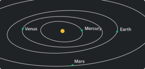
The planets move through space in elliptical, periodic orbits about the sun, as shown in Figure 1. They are in constant motion, so fixing an exact position of any planet is valid only for a moment. In other words, we can fix only a planet’s instantaneous position. This is one application of polar coordinates, represented as [latex]\left(r,\theta \right)[/latex]. We interpret [latex]r[/latex] as the distance from the sun and [latex]\theta[/latex] as the planet’s angular bearing, or its direction from a fixed point on the sun. In this section, we will focus on the polar system and the graphs that are generated directly from polar coordinates.
Testing Polar Equations for Symmetry
Just as a rectangular equation such as [latex]y={x}^{2}[/latex] describes the relationship between [latex]x[/latex] and [latex]y[/latex] on a Cartesian grid, a polar equation describes a relationship between [latex]r[/latex] and [latex]\theta[/latex] on a polar grid. Recall that the coordinate pair [latex]\left(r,\theta \right)[/latex] indicates that we move counterclockwise from the polar axis (positive x-axis) by an angle of [latex]\theta[/latex], and extend a ray from the pole (origin) [latex]r[/latex] units in the direction of [latex]\theta[/latex]. All points that satisfy the polar equation are on the graph.
Symmetry is a property that helps us recognize and plot the graph of any equation. By performing three tests, we will see how to apply the properties of symmetry to polar equations. Further, we will use symmetry (in addition to plotting key points, zeros, and maximums of [latex]r[/latex]) to determine the graph of a polar equation.
This equation exhibits symmetry with respect to the line [latex]\theta =\frac{\pi }{2}[/latex].
In the second test, we consider symmetry with respect to the polar axis ( [latex]x[/latex] -axis). We replace [latex]\left(r,\theta \right)[/latex] with [latex]\left(r,-\theta \right)[/latex] or [latex]\left(-r,\pi -\theta \right)[/latex] to determine equivalency between the tested equation and the original. For example, suppose we are given the equation [latex]r=1 - 2\cos \theta[/latex].
The graph of this equation exhibits symmetry with respect to the polar axis.
In the third test, we consider symmetry with respect to the pole (origin). We replace [latex]\left(r,\theta \right)[/latex] with [latex]\left(-r,\theta \right)[/latex] to determine if the tested equation is equivalent to the original equation. For example, suppose we are given the equation [latex]r=2\sin \left(3\theta \right)[/latex].
The equation has failed the symmetry test, but that does not mean that it is not symmetric with respect to the pole. Passing one or more of the symmetry tests verifies that symmetry will be exhibited in a graph. However, failing the symmetry tests does not necessarily indicate that a graph will not be symmetric about the line [latex]\theta =\frac{\pi }{2}[/latex], the polar axis, or the pole. In these instances, we can confirm that symmetry exists by plotting reflecting points across the apparent axis of symmetry or the pole. Testing for symmetry is a technique that simplifies the graphing of polar equations, but its application is not perfect.
symmetry tests
A polar equation describes a curve on the polar grid. The graph of a polar equation can be evaluated for three types of symmetry.
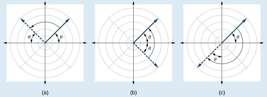
- Substitute the appropriate combination of components for [latex]\left(r,\theta \right):[/latex] [latex]\left(-r,-\theta \right)[/latex] for [latex]\theta =\frac{\pi }{2}[/latex] symmetry; [latex]\left(r,-\theta \right)[/latex] for polar axis symmetry; and [latex]\left(-r,\theta \right)[/latex] for symmetry with respect to the pole.
- If the resulting equations are equivalent in one or more of the tests, the graph produces the expected symmetry.
