- Graph exponential functions.
- Graph exponential functions using transformations.
Exponential functions are used for many real-world applications such as finance, forensics, computer science, and most of the life sciences. Working with an equation that describes a real-world situation gives us a method for making predictions. Most of the time, however, the equation itself is not enough. We learn a lot about things by seeing their pictorial representations, and that is exactly why graphing exponential equations is a powerful tool. It gives us another layer of insight for predicting future events.
Defining Exponential Functions
What exactly does it mean to grow exponentially? What does the word double have in common with percent increase? People toss these words around errantly. Are these words used correctly? The words certainly appear frequently in the media.
- Percent change refers to a change based on a percent of the original amount.
- Exponential growth refers to an increase based on a constant multiplicative rate of change over equal increments of time, that is, a percent increase of the original amount over time.
- Exponential decay refers to a decrease based on a constant multiplicative rate of change over equal increments of time, that is, a percent decrease of the original amount over time.
For us to gain a clear understanding of exponential growth, let us contrast exponential growth with linear growth.
| [latex]x[/latex] | [latex]y = 2^x[/latex] | [latex]y = 2x[/latex] |
| [latex]0[/latex] | [latex]y = 2^0 = 1[/latex] | [latex]y = 2(0) = 0[/latex] |
| [latex]1[/latex] | [latex]y = 2^1 = 2[/latex] | [latex]y = 2(1) = 2[/latex] |
| [latex]2[/latex] | [latex]y = 2^2 = 4[/latex] | [latex]y = 2(2) = 4[/latex] |
| [latex]3[/latex] | [latex]y = 2^3 = 8[/latex] | [latex]y = 2(3) = 6[/latex] |
| [latex]4[/latex] | [latex]y = 2^4 = 16[/latex] | [latex]y = 2(4) = 8[/latex] |
We can infer that for these two functions, exponential growth dwarfs linear growth.
- Exponential growth refers to the original value from the range increases by the same percentage over equal increments found in the domain.
- Linear growth refers to the original value from the range increases by the same amount over equal increments found in the domain.
Apparently, the difference between “the same percentage” and “the same amount” is quite significant. For exponential growth, over equal increments, the constant multiplicative rate of change resulted in doubling the output whenever the input increased by one. For linear growth, the constant additive rate of change over equal increments resulted in adding [latex]2[/latex] to the output whenever the input was increased by one.
exponential function
The general form of the exponential formula is
[latex]f(x)=ab^x[/latex]
where [latex]a[/latex] is any nonzero number and [latex]b[/latex] is a positive real number not equal to [latex]1[/latex].
- if [latex]b>1[/latex], the function grows at a rate proportional to its size.
- if [latex]0 \lt b \lt 1[/latex], the function decays at a rate proportional to its size.
This is done to ensure that the outputs will be real numbers. Observe what happens if the base is not positive:
- Consider a base of –9 and exponent of [latex]\frac{1}{2}[/latex]. Then [latex]f\left(x\right)=f\left(\frac{1}{2}\right)={\left(-9\right)}^{\frac{1}{2}}=\sqrt{-9}[/latex], which is not a real number.
Why do we limit the base to positive values other than 1?
This is because a base of 1 results in the constant function. Observe what happens if the base is 1:
- Consider a base of 1. Then [latex]f\left(x\right)={1}^{x}=1[/latex] for any value of x.
Exponential Growth
Because the output of exponential functions increases very rapidly, the term “exponential growth” is often used in everyday language to describe anything that grows or increases rapidly. However, exponential growth can be defined more precisely in a mathematical sense. If the growth rate is proportional to the amount present, the function models exponential growth.
To get a sense of the behavior of exponential growth, we can create a table of values for a function of the form [latex]f(x)={b}^{x}[/latex], where [latex]f \gt 1[/latex].
| [latex]x[/latex] | [latex]–3[/latex] | [latex]–2[/latex] | [latex]–1[/latex] | [latex]0[/latex] | [latex]1[/latex] | [latex]2[/latex] | [latex]3[/latex] |
| [latex]f\left(x\right)={2}^{x}[/latex] | [latex]\frac{1}{8}[/latex] | [latex]\frac{1}{4}[/latex] | [latex]\frac{1}{2}[/latex] | [latex]1[/latex] | [latex]2[/latex] | [latex]4[/latex] | [latex]8[/latex] |
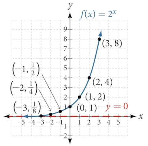 We call the base [latex]2[/latex] the constant ratio. This means that as the input increases by [latex]1[/latex], the output value will be the product of the base and the previous output. Did you notice that the next number is [latex]2[/latex] times the previous number?
This pattern shows exponential growth because the output value increases by a factor of [latex]2[/latex] each time.
Characteristics:
- Domain: [latex](-\infty,\infty)[/latex]
- Range: [latex](0,\infty)[/latex]
- As [latex]x \rightarrow \infty, f(x) \rightarrow \infty[/latex].
- As [latex]x \rightarrow -\infty, f(x) \rightarrow 0[/latex].
- the graph of [latex]f[/latex] will never touch the [latex]x[/latex]-axis because base two raised to any exponent never has the result of zero.
- Horizontal Asymptote: [latex]y = 0[/latex]
- [latex]f(x)[/latex] is always increasing.
- No [latex]x[/latex]-intercept.
- [latex]y[/latex]-intercept is [latex](0,1)[/latex].
exponential growth
A function that models exponential growth grows by a rate proportional to the amount present. For any real number [latex]x[/latex] and any positive real numbers a and b such that [latex]b\ne 1[/latex], an exponential growth function has the form
[latex]\text{ }f\left(x\right)=a{b}^{x}[/latex]
where
- [latex]a[/latex] is the initial or starting value of the function.
- [latex]b[/latex] is the growth factor or growth multiplier per unit [latex]x[/latex].
In more general terms, an exponential function consists of a constant base raised to a variable exponent.
- Company A has [latex]100[/latex] stores and expands by opening [latex]50[/latex] new stores a year, so its growth can be represented by the function [latex]A\left(x\right)=100+50x[/latex].
- Company B has [latex]100[/latex] stores and expands by increasing the number of stores by [latex]50 \%[/latex] each year, so its growth can be represented by the function [latex]B\left(x\right)=100{\left(1+0.5\right)}^{x}[/latex].
A few years of growth for these companies are illustrated below.
| Year, [latex]x[/latex] | Stores, Company A | Stores, Company B |
|---|---|---|
| [latex]0[/latex] | [latex]100 + 50(0) = 100[/latex] | [latex]100(1 + 0.5)^0 = 100[/latex] |
| [latex]1[/latex] | [latex]100 + 50(1) = 150[/latex] | [latex]100(1 + 0.5)^1 = 150[/latex] |
| [latex]2[/latex] | [latex]100 + 50(2) = 200[/latex] | [latex]100(1 + 0.5)^2 = 225[/latex] |
| [latex]3[/latex] | [latex]100 + 50(3) = 250[/latex] | [latex]100(1 + 0.5)^3 = 337.5[/latex] |
| [latex]x[/latex] | [latex]A(x) = 100 + 50x[/latex] | [latex]B(x) = 100(1 + 0.5)^x[/latex] |
The graphs comparing the number of stores for each company over a five-year period are shown below. We can see that, with exponential growth, the number of stores increases much more rapidly than with linear growth.
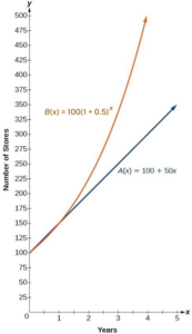
Notice that the domain for both functions is [latex]\left[0,\infty \right)[/latex], and the range for both functions is [latex]\left[100,\infty \right)[/latex]. After year 1, Company B always has more stores than Company A.
Let’s more closely examine the function representing the number of stores for Company B,
In this exponential function, [latex]100[/latex] represents the initial number of stores, [latex]0.5[/latex] represents the growth rate, and [latex]1+0.5=1.5[/latex] represents the growth factor. Generalizing further, we can write this function as
where [latex]100[/latex] is the initial value, [latex]1.5[/latex] is called the base, and [latex]x[/latex] is called the exponent.
[latex]\\[/latex]
This situation is represented by the growth function [latex]P\left(t\right)=1.25{\left(1.012\right)}^{t}[/latex] where [latex]t[/latex] is the number of years since 2013.
[latex]\\[/latex]
To the nearest thousandth, what will the population of India be in 2031?
Exponential Decay
To get a sense of the behavior of exponential decay, we can create a table of values for a function of the form [latex]g(x)={b}^{x}[/latex], where [latex]0 \lt b \lt 1[/latex].
| [latex]x[/latex] | [latex]–3[/latex] | [latex]–2[/latex] | [latex]–1[/latex] | [latex]0[/latex] | [latex]1[/latex] | [latex]2[/latex] | [latex]3[/latex] |
| [latex]g(x)=(\frac{1}{2})^{x}[/latex] | [latex]8[/latex] | [latex]4[/latex] | [latex]2[/latex] | [latex]1[/latex] | [latex]\frac{1}{2}[/latex] | [latex]\frac{1}{4}[/latex] | [latex]\frac{1}{8}[/latex] |
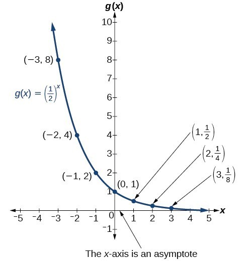 When the input is increasing by [latex]1[/latex], each output value is the product of the previous output and the base or constant ratio [latex]\frac{1}{2}[/latex].
Notice from the table that:
- the output values are positive for all values of [latex]x[/latex].
- as [latex]x[/latex] increases, the output values grow smaller, approaching zero.
- as [latex]x[/latex] decreases, the output values grow without bound.
Characteristics:
- Domain: [latex]\left(-\infty , \infty \right)[/latex]
- Range: [latex]\left(0,\infty \right)[/latex]
- [latex]x[/latex]–intercept: none
- [latex]y[/latex]–intercept: [latex]\left(0,1\right)[/latex]
- Horizontal asymptote: [latex]y=0[/latex]
This is an exponential decay.