Graph exponential functions
characteristics of the graph of the parent function [latex]f\left(x\right)={b}^{x}[/latex]
An exponential function with the form [latex]f\left(x\right)={b}^{x}[/latex], [latex]b>0[/latex], [latex]b\ne 1[/latex], has these characteristics:
- one-to-one function
- The horizontal asymptote is [latex]y = 0[/latex].
- The domain of [latex]f[/latex] is all real numbers, [latex](-\infty, \infty)[/latex].
- The range of [latex]f[/latex] is all positive real numbers, [latex](0, \infty)[/latex].
- There is no [latex]x[/latex]-intercept.
- The [latex]y[/latex]-intercept is [latex]\left(0,1\right)[/latex].
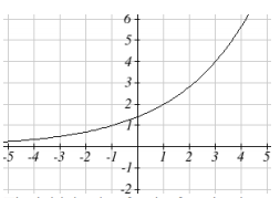
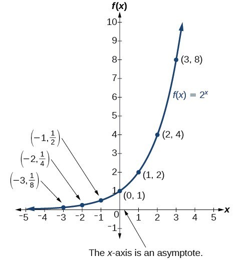
- The graph is increasing if [latex]b \gt 1[/latex], which implies exponential growth.
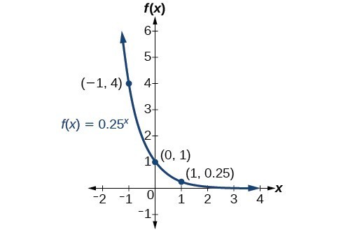
- The graph decreasing if [latex]0 \lt b \lt 1[/latex], which implies exponential decay.
- Create a table of points.
- Plot at least [latex]3[/latex] point from the table including the y-intercept [latex]\left(0,1\right)[/latex].
- Draw a smooth curve through the points.
- State the domain, [latex]\left(-\infty ,\infty \right)[/latex], the range, [latex]\left(0,\infty \right)[/latex], and the horizontal asymptote, [latex]y=0[/latex].
[latex]\\[/latex]
With few exceptions, such as functions that would be undefined at zero or negative input like the radical or (as you’ll see soon) the logarithmic function, it is good practice to let the input equal [latex]-3, -2, -1, 0, 1, 2, \text{ and } 3[/latex] to get the idea of the shape of the graph.
Exponential Growth vs. Decay
The graph of exponential growth is increasing like shown in the graph below.
The graph of the exponential decay function, [latex]g\left(x\right)={\left(\frac{1}{2}\right)}^{x}[/latex] decreases, but with a similar (reflected) shape.
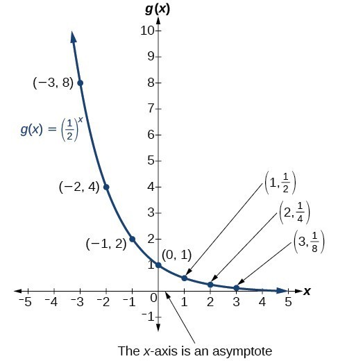
The domain of [latex]g\left(x\right)={\left(\frac{1}{2}\right)}^{x}[/latex] is all real numbers, the range is [latex]\left(0,\infty \right)[/latex], and the horizontal asymptote is [latex]y=0[/latex].