Linear Growth
In the previous example, Marco’s collection grew by the same number of bottles every year. This constant change is the defining characteristic of linear growth. Plotting the values we calculated for Marco’s collection, we can see the values form a straight line, the shape of linear growth.
linear growth
If a quantity starts at size [latex]P_0[/latex] and grows by [latex]d[/latex] every time period, then the quantity after [latex]n[/latex] time periods can be determined using either of these relations:
Recursive form
[latex]P_n = P_{n-1} + d[/latex]
Explicit form
[latex]P_n = P_0 + d n[/latex]
In this equation, [latex]d[/latex] represents the common difference – the amount that the population changes each time [latex]n[/latex] increases by [latex]1[/latex].
You may recognize the common difference, [latex]d[/latex], in our linear equation as slope. In fact, the entire explicit equation should look familiar – it is the same linear equation you learned in algebra, probably stated as [latex]y = mx + b[/latex].
In the standard algebraic equation [latex]y = mx + b[/latex], [latex]b[/latex] was the y-intercept, or the [latex]y[/latex] value when [latex]x[/latex] was zero. In the form of the equation we’re using, we are using [latex]P_0[/latex] to represent that initial amount.
In the [latex]y = mx + b[/latex] equation, recall that [latex]m[/latex] was the slope. You might remember this as “rise over run,” or the change in [latex]y[/latex] divided by the change in [latex]x[/latex]. Either way, it represents the same thing as the common difference, [latex]d[/latex], we are using – the amount the output [latex]P_n[/latex] changes when the input [latex]n[/latex] increases by [latex]1[/latex].
The equations [latex]y = mx + b[/latex] and [latex]P_n = P_0 + d n[/latex] mean the same thing and can be used the same ways. We’re just writing it somewhat differently.
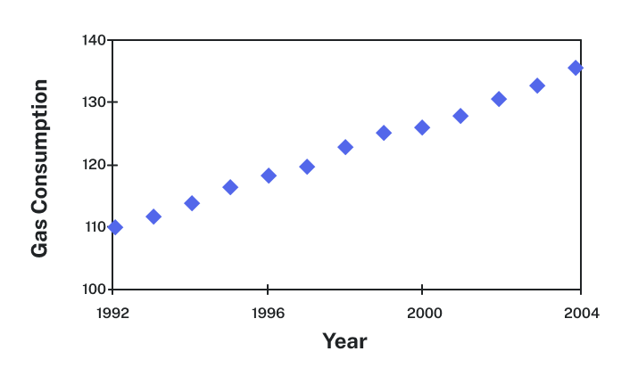
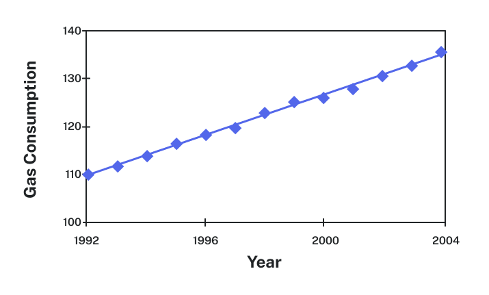
| Year | ’92 | ’93 | ’94 | ’95 | ’96 | ’97 | ’98 | ’99 | ’00 | ’01 | ’02 | ’03 | ’04 |
| Consumption (billion of gallons) | [latex]110[/latex] | [latex]111[/latex] | [latex]113[/latex] | [latex]116[/latex] | [latex]118[/latex] | [latex]119[/latex] | [latex]123[/latex] | [latex]125[/latex] | [latex]126[/latex] | [latex]128[/latex] | [latex]131[/latex] | [latex]133[/latex] | [latex]136[/latex] |
When Good Models Go Bad
Recursive form
[latex]P_0 = 39[/latex]
[latex]P_n = P_{n-1} + 2.5[/latex]
Explicit form
[latex]P_n = 39 + 2.5 n[/latex]
So at 6 years old, we would expect him to be
[latex]P_2 = 39 + 2.5(2) = 44[/latex] inches tall
Any mathematical model will break down eventually. Certainly, we shouldn’t expect this boy to continue to grow at the same rate all his life. If he did, at age 50 he would be
[latex]P_{46} = 39 + 2.5(46) = 154[/latex] inches tall [latex]= 12.8[/latex] feet tall!
When using any mathematical model, we have to consider which inputs are reasonable to use. Whenever we extrapolate, or make predictions into the future, we are assuming the model will continue to be valid.
View a video explanation of this breakdown of the linear growth model here.
You can view the transcript for “Linear model breakdown” here (opens in new window).
- "https://www.bts.gov/archive/publications/national_transportation_statistics/2005/table_04_10". ↵