With Hamiltonian circuits, our focus will not be on existence, but on the question of optimization; given a graph where the edges have weights, can we find the optimal Hamiltonian circuit; the one with lowest total weight.
This problem is called the Traveling salesperson problem (TSP) because the question can be framed like this: Suppose a salesperson needs to give sales pitches in four cities. They looks up the airfares between each city, and put the costs in a graph. The salesperson needs to figure out what order they should travel to visit each city once then return home with the lowest cost?
To answer this question of how to find the lowest cost Hamiltonian circuit, we will consider some possible approaches.
Brute Force Algorithm
The first option that might come to mind is to just try all different possible circuits. We call this the brute force algorithm.
How To: Brute Force Algorithm (a.k.a. exhaustive search)
- List all possible Hamiltonian circuits
- Find the length of each circuit by adding the edge weights
- Select the circuit with minimal total weight.
The Brute force algorithm is optimal; it will always produce the Hamiltonian circuit with minimum weight. Is it efficient? To answer that question, we need to consider how many Hamiltonian circuits a graph could have. For simplicity, let’s look at the worst-case possibility, where every vertex is connected to every other vertex. This is called a complete graph.
Suppose we had a complete graph with five vertices like the air travel graph above. From Seattle there are four cities we can visit first. From each of those, there are three choices. From each of those cities, there are two possible cities to visit next. There is then only one choice for the last city before returning home. This can be shown visually:
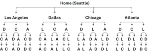
Counting the number of routes, we can see there are [latex]4\cdot{3}\cdot{2}\cdot{1}[/latex] routes. For six cities there would be [latex]5\cdot{4}\cdot{3}\cdot{2}\cdot{1}[/latex] routes.
Number of Possible Circuits
For [latex]N[/latex] vertices in a complete graph, there will be [latex](n-1)!=(n-1)(n-2)(n-3)\dots{3}\cdot{2}\cdot{1}[/latex] routes. Half of these are duplicates in reverse order, so there are [latex]\frac{(n-1)!}{2}[/latex] unique circuits.
The exclamation symbol, [latex]![/latex], is read “factorial” and is shorthand for the product shown.
As you can see the number of circuits is growing extremely quickly. If a computer looked at one billion circuits a second, it would still take almost two years to examine all the possible circuits with only [latex]20[/latex] cities! Certainly brute force is not an efficient algorithm. Let’s look at another option.
Nearest Neighbor Algorithm
- Select a starting point.
- Move to the nearest unvisited vertex (the edge with smallest weight).
- Repeat until the circuit is complete.
Unfortunately, no one has yet found an efficient and optimal algorithm to solve the TSP, and it is very unlikely anyone ever will. Since it is not practical to use brute force to solve the problem, we turn instead to heuristic algorithms; efficient algorithms that give approximate solutions. In other words, heuristic algorithms are fast, but may or may not produce the optimal circuit.
Consider again our salesperson.
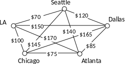
Starting at Seattle, the nearest neighbor (cheapest flight) is to LA, at a cost of [latex]$70[/latex]. From there:
- LA to Chicago: [latex]$100[/latex]
- Chicago to Atlanta: [latex]$75[/latex]
- Atlanta to Dallas: [latex]$85[/latex]
- Dallas to Seattle: [latex]$120[/latex]
- Total cost: [latex]$450[/latex]
In this case, nearest neighbor found the optimal circuit.
What if the NNA does not pick the most optimal edge?
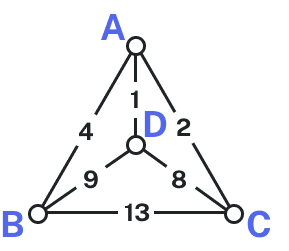
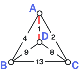
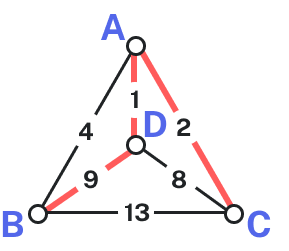
Consider our earlier graph, shown to the right.
Starting at vertex [latex]A[/latex], the nearest neighbor is vertex [latex]D[/latex] with a weight of [latex]1[/latex].
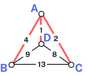
From [latex]D[/latex], the nearest neighbor is [latex]C[/latex], with a weight of [latex]8[/latex].
From [latex]C[/latex], our only option is to move to vertex [latex]B[/latex], the only unvisited vertex, with a cost of [latex]13[/latex].
From [latex]B[/latex] we return to [latex]A[/latex] with a weight of [latex]4[/latex].
The resulting circuit is [latex]ADCBA[/latex] with a total weight of [latex]1+8+13+4 = 26[/latex].
We ended up finding the worst circuit in the graph! What happened? Unfortunately, while it is very easy to implement, the NNA is a greedy algorithm, meaning it only looks at the immediate decision without considering the consequences in the future. In this case, following the edge [latex]AD[/latex] forced us to use the very expensive edge [latex]BC[/latex] later. How could we improve the outcome? One option would be to redo the nearest neighbor algorithm with a different starting point to see if the result changed. Since nearest neighbor is so fast, doing it several times isn’t a big deal.
Starting at vertex [latex]A[/latex] resulted in a circuit with weight [latex]26[/latex], as seen above. Lets repeat the NNA for the other vertices.
Starting at vertex [latex]B[/latex], the nearest neighbor circuit is [latex]BADCB[/latex] with a weight of [latex]4+1+8+13 = 26[/latex]. This is the same circuit we found starting at vertex [latex]A[/latex]. No better.
Starting at vertex [latex]C[/latex], the nearest neighbor circuit is [latex]CADBC[/latex] with a weight of [latex]2+1+9+13 = 25[/latex]. Better!
Starting at vertex [latex]D[/latex], the nearest neighbor circuit is [latex]DACBA[/latex]. Notice that this is actually the same circuit we found starting at [latex]C[/latex], just written with a different starting vertex.
The repeat nearest neighbor algorithm (RNNA) was able to produce a slightly better circuit with a weight of [latex]25[/latex], but still not the optimal circuit in this case. Notice that even though we found the circuit by starting at vertex [latex]C[/latex], we could still write the circuit starting at [latex]A[/latex]: [latex]ADBCA[/latex] or [latex]ACBDA[/latex].
| [latex]A[/latex] | [latex]B[/latex] | [latex]C[/latex] | [latex]D[/latex] | [latex]E[/latex] | [latex]F[/latex] | |
| [latex]A[/latex] | — | [latex]44[/latex] | [latex]34[/latex] | [latex]12[/latex] | [latex]40[/latex] | [latex]41[/latex] |
| [latex]B[/latex] | [latex]44[/latex] | — | [latex]31[/latex] | [latex]43[/latex] | [latex]24[/latex] | [latex]50[/latex] |
| [latex]C[/latex] | [latex]34[/latex] | [latex]31[/latex] | — | [latex]20[/latex] | [latex]39[/latex] | [latex]27[/latex] |
| [latex]D[/latex] | [latex]12[/latex] | [latex]43[/latex] | [latex]20[/latex] | — | [latex]11[/latex] | [latex]17[/latex] |
| [latex]E[/latex] | [latex]40[/latex] | [latex]24[/latex] | [latex]39[/latex] | [latex]11[/latex] | — | [latex]42[/latex] |
| [latex]F[/latex] | [latex]41[/latex] | [latex]50[/latex] | [latex]27[/latex] | [latex]17[/latex] | [latex]42[/latex] | — |
- Find the circuit generated by the NNA starting at vertex [latex]B[/latex].
- Find the circuit generated by the RNNA.
While certainly better than the basic NNA, unfortunately, the RNNA is still greedy and will produce very bad results for some graphs. As an alternative, our next approach will step back and look at the “big picture” – it will select first the edges that are shortest, and then fill in the gaps.
Sorted Edges Algorithm
How To: Sorted Edges Algorithm (a.k.a. cheapest link algorithm)
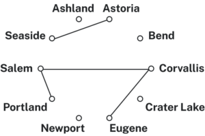
- Select the cheapest unused edge in the graph.
- Repeat step 1, adding the cheapest unused edge to the circuit, unless:
- adding the edge would create a circuit that doesn’t contain all vertices, or
- adding the edge would give a vertex degree [latex]3[/latex].
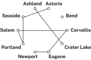
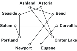
- Repeat until a circuit containing all vertices is formed.
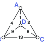
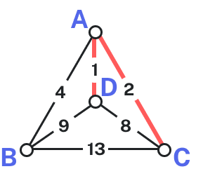
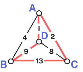
The cheapest edge is [latex]AD[/latex], with a cost of [latex]1[/latex]. We highlight that edge to mark it selected. The next shortest edge is [latex]AC[/latex], with a weight of [latex]2[/latex], so we highlight that edge.
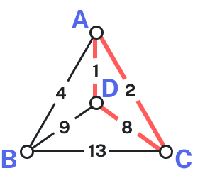
For the third edge, we’d like to add [latex]AB[/latex], but that would give vertex [latex]A[/latex] degree [latex]3[/latex], which is not allowed in a Hamiltonian circuit. The next shortest edge is [latex]CD[/latex], but that edge would create a circuit [latex]ACDA[/latex] that does not include vertex [latex]B[/latex], so we reject that edge. The next shortest edge is [latex]BD[/latex], so we add that edge to the graph.
Bad
Bad
Okay
We then add the last edge to complete the circuit: [latex]ACBDA[/latex] with weight [latex]25[/latex]. Notice that the algorithm did not produce the optimal circuit in this case; the optimal circuit is [latex]ACDBA[/latex] with weight [latex]23[/latex].
While the Sorted Edge algorithm overcomes some of the shortcomings of NNA, it is still only a heuristic algorithm, and does not guarantee the optimal circuit.
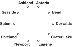
| Ashland | Astoria | Bend | Corvallis | Crater Lake | Eugene | Newport | Portland | Salem | Seaside | |
| Ashland | – | [latex]374[/latex] | [latex]200[/latex] | [latex]223[/latex] | [latex]108[/latex] | [latex]178[/latex] | [latex]252[/latex] | [latex]285[/latex] | [latex]240[/latex] | [latex]356[/latex] |
| Astoria | [latex]374[/latex] | – | [latex]255[/latex] | [latex]166[/latex] | [latex]433[/latex] | [latex]199[/latex] | [latex]135[/latex] | [latex]95[/latex] | [latex]136[/latex] | [latex]17[/latex] |
| Bend | [latex]200[/latex] | [latex]255[/latex] | – | [latex]128[/latex] | [latex]277[/latex] | [latex]128[/latex] | [latex]180[/latex] | [latex]160[/latex] | [latex]131[/latex] | [latex]247[/latex] |
| Corvallis | [latex]223[/latex] | [latex]166[/latex] | [latex]128[/latex] | – | [latex]430[/latex] | [latex]47[/latex] | [latex]52[/latex] | [latex]84[/latex] | [latex]40[/latex] | [latex]155[/latex] |
| Crater Lake | [latex]108[/latex] | [latex]433[/latex] | [latex]277[/latex] | [latex]430[/latex] | – | [latex]453[/latex] | [latex]478[/latex] | [latex]344[/latex] | [latex]389[/latex] | [latex]423[/latex] |
| Eugene | [latex]178[/latex] | [latex]199[/latex] | [latex]128[/latex] | [latex]47[/latex] | [latex]453[/latex] | – | [latex]91[/latex] | [latex]110[/latex] | [latex]64[/latex] | [latex]181[/latex] |
| Newport | [latex]252[/latex] | [latex]135[/latex] | [latex]180[/latex] | [latex]52[/latex] | [latex]478[/latex] | [latex]91[/latex] | – | [latex]114[/latex] | [latex]83[/latex] | [latex]117[/latex] |
| Portland | [latex]285[/latex] | [latex]95[/latex] | [latex]160[/latex] | [latex]84[/latex] | [latex]344[/latex] | [latex]110[/latex] | [latex]114[/latex] | – | [latex]47[/latex] | [latex]78[/latex] |
| Salem | [latex]240[/latex] | [latex]136[/latex] | [latex]131[/latex] | [latex]40[/latex] | [latex]389[/latex] | [latex]64[/latex] | [latex]83[/latex] | [latex]47[/latex] | – | [latex]118[/latex] |
| Seaside | [latex]356[/latex] | [latex]17[/latex] | [latex]247[/latex] | [latex]155[/latex] | [latex]423[/latex] | [latex]181[/latex] | [latex]117[/latex] | [latex]78[/latex] | [latex]118[/latex] | – |