- Determine whether a graph has an Euler path or circuit and use Fleury’s algorithm to find an Euler circuit
- Recognize whether a graph contains a Hamiltonian circuit or path and determine the optimal Hamiltonian circuit using various algorithms
- Identify a connected graph as a spanning tree and utilize Kruskal’s algorithm to create both a spanning tree and a minimum-cost spanning tree
Euler Circuits
Euler paths and circuits are concepts in graph theory that help us analyze and solve various problems related to networks, routes, and connections. They provide a way to systematically explore graphs and determine the most efficient paths or circuits to visit all edges or vertices.
Euler Path: An Euler path is a path in a graph that visits every edge exactly once. It starts at one vertex and ends at another vertex, but may not necessarily visit all vertices in the graph. In other words, an Euler path allows us to travel through all the edges of a graph without lifting the pen from the paper (or without retracing any edges).
Euler Circuit: An Euler circuit is a special type of Euler path that starts and ends at the same vertex. It visits every edge exactly once and also includes all the vertices in the graph. Similar to an Euler path, an Euler circuit allows us to traverse through all the edges of a graph without lifting the pen and also ensures that we return to the starting point.
You can view the transcript for “Eulerian Circuits and Eulerian Graphs | Graph Theory, Euler Graphs and Euler Circuits” here (opens in new window).
Notice that every vertex in this graph has even degree, so this graph does have an Euler circuit.
The following video gives more examples of how to determine an Euler path, and an Euler Circuit for a graph.
You can view the transcript for “Graph Theory: Euler Paths and Euler Circuits” here (opens in new window).
Fleury’s Algorithm
Fleury’s Algorithm is a method used to find an Eulerian path or circuit in a graph. It helps us determine if a graph has an Euler path or circuit and, if it does, find the specific path or circuit.
The algorithm works by iteratively selecting edges in the graph while ensuring that they do not disconnect the graph or create any bridges (edges that, if removed, would separate the graph into two or more disconnected components). The goal is to visit every edge in the graph exactly once, following a specific set of rules to maintain connectivity.
Fleury’s Algorithm starts at an arbitrary vertex and chooses edges that are not bridges until there are no more available edges. If at any point there are multiple choices, the algorithm selects an edge that does not create a bridge. By carefully selecting edges in this way, the algorithm constructs an Eulerian path or circuit that covers all edges of the graph.
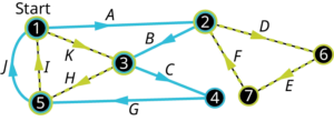
Another method of identifying Euler circuits is to find any circuit in the graph, then find a second circuit starting at a vertex from the first circuit that uses only edges that were not in the first circuit, then find a third circuit starting at a vertex from either of the first two circuits that uses only edges that were not in the first two circuits, and then continue this process until all edges have been used. In the end, you will be able to link all the circuits together into one large Euler circuit. Let’s find an Euler circuit in the map of the Camp Woebegone canoe race. In the figure below, we have labeled the edges of the multigraph so that the circuits can be named. In a multigraph it is necessary to name circuits using edges and vertices because there can be more than one edge between adjacent vertices.
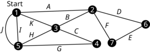
We will begin with vertex [latex]1[/latex] because it represents the starting line in this application. In general, you can start at any vertex you want. Find any circuit beginning and ending with vertex 1. Remember, a circuit is a trail, so it doesn’t pass through any edge more than once. The figure below shows one possible circuit that we could use as the first circuit, [latex]1 → A → 2 → B → 3 → C → 4 → G → 5 → J → 1[/latex].
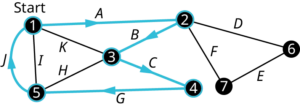
From the edges that remain, we can form two more circuits that each start at one of the vertices along the first circuit. Starting at vertex [latex]3[/latex] we can use [latex]3 → H → 5 → I → 1 → K → 3[/latex] and starting at vertex [latex]2[/latex] we can use [latex]2 → D → 6 → E → 7 → F → 2[/latex], as shown below.
Now that each of the edges is included in one and only once circuit, we can create one large circuit by inserting the second and third circuits into the first. We will insert them at their starting vertices 2 and 3
becomes
Finally, we can name the circuit using vertices, [latex]1 → 2 → 6 → 7 → 2 → 3 → 5 → 1 → 3 → 4 → 5 → 1,[/latex] or edges, [latex]A → D → E → F → B → H → I → K → C → G → J[/latex].
Let’s review the steps we used to find this Eulerian Circuit.
Steps to Find an Euler Circuit in an Eulerian Graph
- Step 1: Find a circuit beginning and ending at any point on the graph. If the circuit crosses every edges of the graph, the circuit you found is an Euler circuit. If not, move on to step 2.
- Step 2: Beginning at a vertex on a circuit you already found, find a circuit that only includes edges that have not previously been crossed. If every edge has been crossed by one of the circuits you have found, move on to Step 3. Otherwise, repeat Step 2.
- Step 3: Now that you have found circuits that cover all of the edges in the graph, combine them into an Euler circuit. You can do this by inserting any of the circuits into another circuit with a common vertex repeatedly until there is one long circuit.
You can view the transcript for “Euler Part 3: Fleury’s Algorithm for Finding an Euler Circuit in Graph with Vertices of Even Degree” here (opens in new window).
Eulerization
Eulerization is the process of modifying a graph by adding edges to make it possible to find an Eulerian circuit or path. It is used when the original graph does not have an Eulerian circuit or path, but we want to transform it in such a way that it becomes possible to traverse all edges exactly once.
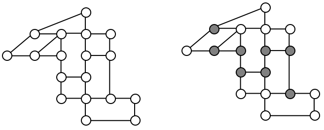
To Eulerize a graph, additional edges are added strategically to connect pairs of vertices with odd degrees. By adding these extra edges, the degrees of all vertices in the modified graph become even, allowing for the existence of an Eulerian circuit or path.
You can view the transcript for “Graph Theory: Eulerization” here (opens in new window).
Hamiltonian Circuits and Paths
Hamiltonian Circuit: A Hamiltonian circuit is a path in a graph that visits every vertex exactly once, starting and ending at the same vertex. In other words, it is a closed loop that passes through every vertex of the graph without revisiting any vertex.
Hamiltonian Path: A Hamiltonian path is a path in a graph that visits every vertex exactly once, but may not necessarily start and end at the same vertex. Unlike a Hamiltonian circuit, it does not form a closed loop.
The search for Hamiltonian circuits and paths is often considered more difficult than the search for Eulerian circuits and paths, as there is no known general method to quickly find them in arbitrary graphs.
Watch the following video for more information on Hamiltonian circuits and paths.
You can view the transcript for “Graph Theory: Hamiltonian Circuits and Paths” here (opens in new window).
Watch the following video to see examples of finding a Hamiltonian circuit.
You can view the transcript for “Hamiltonian circuits” here (opens in new window).
Brute Force Algorithm
The brute force algorithm is a straightforward and exhaustive approach to problem-solving that involves systematically checking all possible solutions to find the optimal or desired solution. It is called “brute force” because it explores every possible option without using any shortcuts or optimization techniques. This method guarantees finding the correct solution, but it can be computationally intensive and time-consuming, especially for problems with large input sizes. The steps of using the brute force algorithm are:
- List all possible Hamiltonian circuits
- Find the length of each circuit by adding the edge weights
- Select the circuit with minimal total weight.
You can view the transcript for “Graph Theory: The Brute Force Algorithm” here (opens in new window).
Nearest Neighbor Algorithm
The nearest neighbor algorithm is a simple and intuitive approach used to solve certain optimization problems, especially those involving finding the shortest path or tour in a graph. It works by iteratively selecting the nearest unvisited neighbor from the current location until all nodes are visited. The algorithm starts at an arbitrary node and keeps track of the current location. It then selects the closest unvisited neighboring node and moves to that node. This process is repeated until all nodes have been visited, forming a complete tour or path. The steps of using the nearest neighbor algorithm are:
- Select a starting point.
- Move to the nearest unvisited vertex (the edge with smallest weight).
- Repeat until the circuit is complete.
You can view the transcript for “Graph Theory: Nearest Neighbor Algorithm (NNA)” here (opens in new window).
Sorted Edges Algorithm
The sorted edges algorithm is a method used to determine the order in which edges are selected and processed in a graph. It involves sorting the edges of the graph based on a certain criterion, such as their weights, and then iteratively considering these edges in the sorted order. The algorithm starts by sorting all the edges of the graph based on a specific attribute, such as their weights or costs. Once the edges are sorted, they can be processed one by one in the specified order. The steps of using the sorted edges algorithm are:
- Select the cheapest unused edge in the graph.
- Repeat step 1, adding the cheapest unused edge to the circuit, unless:
- adding the edge would create a circuit that doesn’t contain all vertices, or
- adding the edge would give a vertex degree [latex]3[/latex].
- Repeat until a circuit containing all vertices is formed.
You can view the transcript for “Graph Theory: Sorted Edges Algorithm (Cheapest Link Algorithm)” here (opens in new window).
Spanning Trees
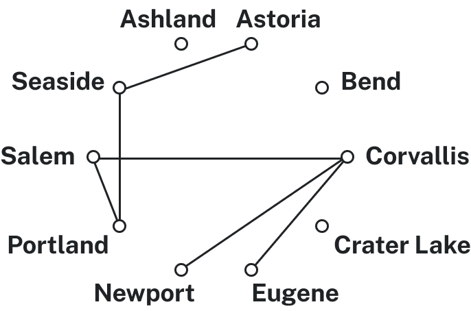
A spanning tree is a subgraph of a connected graph that includes all the vertices of the original graph and forms a tree structure without any cycles.
In other words, it is a tree-like subset of the graph that spans across all the vertices while maintaining connectivity.
A spanning tree can be thought of as a way to connect all the vertices of a graph using the fewest possible number of edges. It eliminates any redundant or unnecessary edges that could form cycles and ensures that there is a unique path between any pair of vertices.
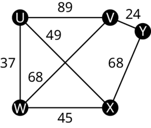
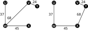
Kruskal’s Algorithm is a popular method used to find a minimum spanning tree in a weighted graph. It efficiently selects edges from the graph based on their weights, gradually forming a minimum spanning tree that connects all the vertices. The steps of using the Kruskal’s Algorithm are:
- Select the cheapest unused edge in the graph.
- Repeat step 1, adding the cheapest unused edge, unless:
- adding the edge would create a circuit
Repeat until a spanning tree is formed
You can view the transcript for “Recognizing and Finding Spanning Trees in Graph Theory” here (opens in new window).
| Ashland | Astoria | Bend | Corvallis | Crater Lake | Eugene | Newport | Portland | Salem | Seaside | |
| Ashland | – | [latex]374[/latex] | [latex]200[/latex] | [latex]223[/latex] | [latex]108[/latex] | [latex]178[/latex] | [latex]252[/latex] | [latex]285[/latex] | [latex]240[/latex] | [latex]356[/latex] |
| Astoria | [latex]374[/latex] | – | [latex]255[/latex] | [latex]166[/latex] | [latex]433[/latex] | [latex]199[/latex] | [latex]135[/latex] | [latex]95[/latex] | [latex]136[/latex] | [latex]17[/latex] |
| Bend | [latex]200[/latex] | [latex]255[/latex] | – | [latex]128[/latex] | [latex]277[/latex] | [latex]128[/latex] | [latex]180[/latex] | [latex]160[/latex] | [latex]131[/latex] | [latex]247[/latex] |
| Corvallis | [latex]223[/latex] | [latex]166[/latex] | [latex]128[/latex] | – | [latex]430[/latex] | [latex]47[/latex] | [latex]52[/latex] | [latex]84[/latex] | [latex]40[/latex] | [latex]155[/latex] |
| Crater Lake | [latex]108[/latex] | [latex]433[/latex] | [latex]277[/latex] | [latex]430[/latex] | – | [latex]453[/latex] | [latex]478[/latex] | [latex]344[/latex] | [latex]389[/latex] | [latex]423[/latex] |
| Eugene | [latex]178[/latex] | [latex]199[/latex] | [latex]128[/latex] | [latex]47[/latex] | [latex]453[/latex] | – | [latex]91[/latex] | [latex]110[/latex] | [latex]64[/latex] | [latex]181[/latex] |
| Newport | [latex]252[/latex] | [latex]135[/latex] | [latex]180[/latex] | [latex]52[/latex] | [latex]478[/latex] | [latex]91[/latex] | – | [latex]114[/latex] | [latex]83[/latex] | [latex]117[/latex] |
| Portland | [latex]285[/latex] | [latex]95[/latex] | [latex]160[/latex] | [latex]84[/latex] | [latex]344[/latex] | [latex]110[/latex] | [latex]114[/latex] | – | [latex]47[/latex] | [latex]78[/latex] |
| Salem | [latex]240[/latex] | [latex]136[/latex] | [latex]131[/latex] | [latex]40[/latex] | [latex]389[/latex] | [latex]64[/latex] | [latex]83[/latex] | [latex]47[/latex] | – | [latex]118[/latex] |
| Seaside | [latex]356[/latex] | [latex]17[/latex] | [latex]247[/latex] | [latex]155[/latex] | [latex]423[/latex] | [latex]181[/latex] | [latex]117[/latex] | [latex]78[/latex] | [latex]118[/latex] | – |