Critical Path Algorithm Cont.
How To: Critical Path Algorithm (version 2)
- Apply the backflow algorithm to the digraph.
- Create the priority list by listing the tasks in order from longest critical time to shortest critical time.
This version of the Critical Path Algorithm will usually be the easier to implement.
Applying this to our digraph from the earlier example, we start applying the backflow algorithm.
Solution
We add an end vertex and give it a critical time of [latex]0[/latex].

We then move back to [latex]T_4,T_9,[/latex] and [latex]T_{10}[/latex], labeling them with their critical times.
![a directed graph with 11 nodes and directed edges connecting them. Each node is labeled T1 to T10, with one end node, with a number in parentheses that could represent a time stamp or identifier. From the top left to the right and then down, the nodes and their connections are as follows: T1(6) has an arrow pointing to T5(5). T5(5) has arrows pointing to both T9(2), T10(7) and T8(3). T9(2) points towards the end node and has [2] next to it. T2(3) has an arrow pointing to T6(10). T6(10) has arrows pointing to both T5(5) and T7(4). T8(3) has an arrow pointing to T10(7). T10(7) is pointing towards the end node and has [7] next to it. T3(7) has an arrow pointing to T7(4). T7(4) has an arrow pointing to T10(7). T4(4) is pointing towards the end node and has [4] next to it. The end node has [0] next to it. The graph may represent a process flow, task dependencies in a project, or transactions in a database system.](https://math.libretexts.org/@api/deki/files/39345/sc11.svg?revision=1&size=bestfit&width=442&height=237)
From each vertex marked with a critical time, we go back. [latex]T_7[/latex], for example, will get labeled with a critical time [latex]11[/latex] – the task time of [latex]4[/latex] plus the critical time of [latex]7[/latex] for [latex]T_{10}[/latex]. For [latex]T_5[/latex], there are two paths to the end. We use the longer, labeling [latex]T_5[/latex] with critical time [latex]5+7=12[/latex].
![a directed graph with 11 nodes and directed edges connecting them. Each node is labeled T1 to T10, with one end node, with a number in parentheses that could represent a time stamp or identifier. From the top left to the right and then down, the nodes and their connections are as follows: T1(6) has an arrow pointing to T5(5). T5(5) has [12] next to it and has arrows pointing to both T9(2), T10(7) and T8(3). T9(2) points towards the end node and has [2] next to it. T2(3) has an arrow pointing to T6(10). T6(10) has arrows pointing to both T5(5) and T7(4). T8(3) has an arrow pointing to T10(7) and has [10] next to it. T10(7) is pointing towards the end node and has [7] next to it. T3(7) has an arrow pointing to T7(4). T7(4) has an arrow pointing to T10(7) and has [14] next to it. T4(4) is pointing towards the end node and has [4] next to it. The end node has [0] next to it. The graph may represent a process flow, task dependencies in a project, or transactions in a database system.](https://math.libretexts.org/@api/deki/files/39346/sc12.svg?revision=1&size=bestfit&width=436&height=233)
Continue the process until all vertices are labeled. Notice that the critical time for [latex]T_5[/latex] ended got replaced later with the even longer path through [latex]T_8[/latex].
![a directed graph with 11 nodes and directed edges connecting them. Each node is labeled T1 to T10, with one end node, with a number in parentheses that could represent a time stamp or identifier. From the top left to the right and then down, the nodes and their connections are as follows: T1(6) has an arrow pointing to T5(5). T5(5) has arrows pointing to both T9(2), T10(7) and T8(3). T9(2) points towards the end node. T10(7) points towards the end node. T2(3) has an arrow pointing to T6(10). T6(10) has arrows pointing to both T5(5) and T7(4). T8(3) has an arrow pointing to T10(7). T3(7) has an arrow pointing to T7(4). T7(4) has an arrow pointing to T10(7). T4(4) is pointing towards the end node. Next to T1(6) is [21], next to T5(5) is [15], next to T9(2) is [2], next to T2(3) is [28], next to T6(10) is [25], next to T8(3) is [10], next to T10(7) is [7], next to T3(7) is [21], next to T7(4) is [14], next to T4(4) is [4], and finally next to the end node is [0].The graph may represent a process flow, task dependencies in a project, or transactions in a database system.](https://math.libretexts.org/@api/deki/files/39347/sc13.svg?revision=1&size=bestfit&width=435&height=245)
We can now quickly create the critical path priority list by listing the tasks in decreasing order of critical time:
Priority list: [latex]T_2,T_6,T_1,T_3,T_5,T_7,T_8,T_{10},T_4,T_9[/latex]
Applying this priority list using the list processing algorithm, we get the schedule:
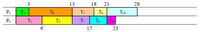
In this particular case, we were able to achieve the minimum possible completion time with this schedule, suggesting that this schedule is optimal. This is certainly not always the case.
In most cases the critical path algorithm will lead to a very good schedule. There are cases where it will not. Unfortunately, there is no known algorithm to always produce the optimal schedule.