Euler and Hamiltonian Paths and Circuits: Apply It 1

  • Determine whether a graph has an Euler path or circuit and use Fleury’s algorithm to find an Euler circuit
  • Recognize whether a graph contains a Hamiltonian circuit or path and determine the optimal Hamiltonian circuit using various algorithms
  • Identify a connected graph as a spanning tree and utilize Kruskal’s algorithm to create both a spanning tree and a minimum-cost spanning tree

Mission Route Optimization

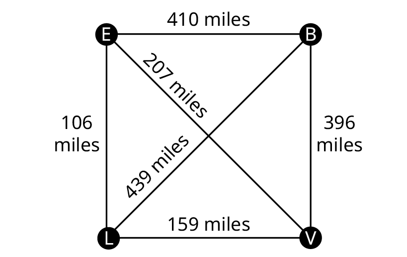
An officer at Vandenberg AFB has a critical assignment that requires visiting three other California Air Force bases: Travis AFB (in Los Angeles), Beale AFB, and Edwards AFB. The officer must determine the most efficient route to visit each base once before returning to Vandenberg. The vertices in the graph below represent the four U.S. Air Force bases, Vandenberg, Edwards, Los Angeles, and Beale. The edges are labeled to with the driving distance between each pair of cities.

A graph represents the four California air force bases. The graph has four vertices: E, B, V, and L. The edge, E B is labeld 410 miles. The edge, B V is labeled 396 miles. The edge, V L is labeled 159 miles. The edge, L E is labeled 106 miles. The edge, L B is labeled 439 miles. The edge, E V is labeled 207 miles.


Before our officer can embark on their mission, it’s essential to understand the underlying structure of the routes between bases. This begins with a fundamental concept in graph theory: the Euler circuit.


Having established the feasibility of an Euler circuit within the network of bases, we shift our focus to planning an actual mission route. A Hamiltonian cycle will ensure that each base is visited just once – a critical requirement for the officer’s itinerary.

Any route that visits each base and returns to the start would be a Hamilton cycle on the graph. Since the distance between bases is the same in either direction, it does not matter if the officer travels clockwise or counterclockwise. So, there are really only three possible distances as shown below.

Three graphs represent the four California air force bases. Each graph has four vertices: E, B, V, and L. The edge, E B is labeled 410 miles. The edge, B V is labeled 396 miles. The edge, V L is labeled 159 miles. The edge, L E is labeled 106 miles. The edge, L B is labeled 439 miles. The edge, E V is labeled 207 miles. In the first graph, the edges, E V, and L B are in dashed lines. In the second graph, the edges, E L and B V are in dashed lines. In the third graph, the edges, E B and L V are in dashed lines.
Three Possible Distances

The officer will now use the strategy of the Traveling Salesperson Problem to determine the most efficient sequence of visits.