Compound Interest vs Simple Interest
Let us compare the amount of money earned from compounding against the amount you would earn from simple interest
| Years | Simple Interest
[latex]$15[/latex] per month |
[latex]6\%[/latex] Annual Rate Compounded Monthly
[latex]0.5\%[/latex] each month |
| [latex]0[/latex] | [latex]$3,000[/latex] | [latex]$3,000[/latex] |
| [latex]5[/latex] | [latex]$3,900[/latex] | [latex]$4,046.55[/latex] |
| [latex]10[/latex] | [latex]$4,800[/latex] | [latex]$5,458.19[/latex] |
| [latex]15[/latex] | [latex]$5,700[/latex] | [latex]$7,362.28[/latex] |
| [latex]20[/latex] | [latex]$6,600[/latex] | [latex]$9,930.61[/latex] |
| [latex]25[/latex] | [latex]$7,500[/latex] | [latex]$13,394.91[/latex] |
| [latex]30[/latex] | [latex]$8,400[/latex] | [latex]$18,067.73[/latex] |
| [latex]35[/latex] | [latex]$9,300[/latex] | [latex]$24,370.65[/latex] |
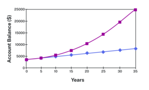
As you can see, over a long period of time, compounding makes a large difference in the account balance. You may recognize this as the difference between linear growth and exponential growth.
Linear growth vs exponential growth
Recall that linear growth increases at a constant rate. A graph of linear growth will describe a straight line between any two points on the graph. The graph changes by the same additive amount per unit of input.
For example, a bank account that grows at [latex]$5[/latex] per year experiences linear growth.
Exponential growth describes a quantity growing at a rate proportional to itself for each unit of input. The graph changes by a multiple of its current value per unit of input. The graph will describe a quickly rising curve.
For example, an account that grows at [latex]2\%[/latex] per year experiences exponential growth.
Using a Calculator to Solve Compound Interest
Utilizing a calculator to compute compound interest can streamline the task considerably, but it’s important to approach this tool with a few critical pointers in mind. These include understanding the functions on your calculator, the importance of precision in your inputs, and the nuances of rounding numbers.
How to: Evaluate exponents on the calculator
When we need to calculate something like [latex]5^3[/latex] it is easy enough to just multiply [latex]5\cdot{5}\cdot{5}=125[/latex]. But when we need to calculate something like [latex]1.005^{240}[/latex], it would be very tedious to calculate this by multiplying [latex]1.005[/latex] by itself [latex]240[/latex] times! So to make things easier, we can harness the power of our scientific calculators.
Most scientific calculators have a button for exponents. It is typically either labeled like:
^ , [latex]y^x[/latex] , or [latex]x^y[/latex] .
To evaluate [latex]1.005^{240}[/latex] we’d type [latex]1.005[/latex] ^ [latex]240[/latex], or [latex]1.005 \space{y^{x}}\space 240[/latex]. Try it out – you should get something around [latex]3.3102044758[/latex].
It is important to be very careful about rounding when calculating things with exponents. In general, you want to keep as many decimals during calculations as you can. Be sure to keep at least 3 significant digits (numbers after any leading zeros). Rounding [latex]0.00012345[/latex] to [latex]0.000123[/latex] will usually give you a “close enough” answer, but keeping more digits is always better.
| [latex]P_0 = $1000[/latex] | the initial deposit |
| [latex]r = 0.05[/latex] | [latex]5\%[/latex] |
| [latex]n = 12[/latex] | [latex]12[/latex] months in [latex]1[/latex] year |
| [latex]t = 30[/latex] | since we’re looking for the amount after [latex]30[/latex] years |
If we first compute [latex]\frac{r}{n}[/latex], we find [latex]\frac{0.05}{12} = 0.00416666666667[/latex].
Here is the effect of rounding this to different values:
| [latex]\frac{r}{n}[/latex] rounded to: | Gives [latex]P_{30}[/latex] to be: | Error |
| [latex]0.004[/latex] | [latex]$4208.59[/latex] | [latex]$259.15[/latex] |
| [latex]0.0042[/latex] | [latex]$4521.45[/latex] | [latex]$53.71[/latex] |
| [latex]0.00417[/latex] | [latex]$4473.09[/latex] | [latex]$5.35[/latex] |
| [latex]0.004167[/latex] | [latex]$4468.28[/latex] | [latex]$0.54[/latex] |
| [latex]0.0041667[/latex] | [latex]$4467.80[/latex] | [latex]$0.06[/latex] |
| no rounding | [latex]$4467.74[/latex] |
If you’re working in a bank, of course you wouldn’t round at all. For our purposes, the answer we got by rounding to [latex]0.00417[/latex], three significant digits, is close enough – [latex]$5[/latex] off isn’t too bad. Certainly keeping that fourth decimal place wouldn’t have hurt.
In many cases, you can avoid rounding completely by how you enter things in your calculator.
For example, in the example above, we needed to calculate [latex]{{P}_{30}}=1000{{\left(1+\frac{0.05}{12}\right)}^{12\times30}}[/latex]
We can quickly calculate [latex]12×30 = 360[/latex], giving [latex]{{P}_{30}}=1000{{\left(1+\frac{0.05}{12}\right)}^{360}}[/latex].
Now we can use the calculator.
| Type this | Calculator shows |
| [latex]0.05 ÷ 12 =[/latex] . | [latex]0.00416666666667[/latex] |
| [latex]+ 1 =[/latex] . | [latex]1.00416666666667[/latex] |
| [latex]y^x 360 =[/latex] . | [latex]4.46774431400613[/latex] |
| [latex]× 1000 =[/latex] . | [latex]4467.74431400613[/latex] |
The previous steps were assuming you have a “one operation at a time” calculator; a more advanced calculator will often allow you to type in the entire expression to be evaluated. If you have a calculator like this, you will probably just need to enter: