The Main Idea 

Least Squares Regression (LSR) analysis is a statistical tool that models the strength of a linear relationship between an independent (explanatory) variable and a dependent (response) variable.

A scatterplot is used to display the relationship, in which each data point is a pair of data values, both quantitative, one independent and one dependent. See the image below, depicting quarterly percent change in GDP over quarterly percent change in the unemployment rate. Each data point tells us that, when the percent change in unemployment is some particular amount, the percent change in GDP is a particular corresponding amount. 

 

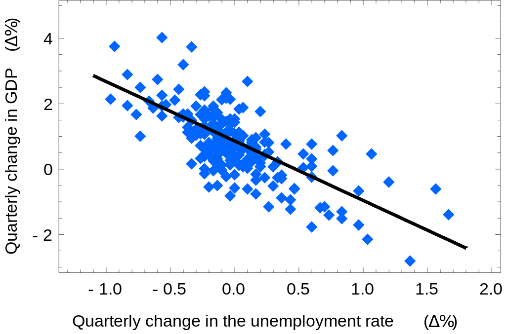
If we think the data on the scatterplot looks even roughly linear, as it does in the graph above, we can try to find a line of best fit using Least Square Regression (LSR). 

Note that LSR can be performed by hand, but you’ll use technology.

The Least Squares Regression analysis produces a line through the dataset that best approximates the linear trend present in the data. It does so by minimizing the sum of the distances between each data point and the line itself.

Vocabulary

• Least Squares Regression, Linear Regression, and Linear Modeling are all terms for the same thing: Finding a line of best fit for a dataset.
• The line of best fit is also called the Least Squares Regression line or the regression line.
• The distance between any data point and the line of best fit is called the residual, or the vertical error of the data point.

The equation of the line of best fit is the equation of a line, [latex]\hat{y}=a+bx[/latex]. The notation [latex]\hat{y}[/latex] is a statistical notation that indicates the output of the equation, the value of the dependent variable, is the general predicted value of the response variable for this linear model.

The correlation coefficient, [latex]r[/latex] tells us how strong the linear relationship is. Values of [latex]r[/latex] very close to [latex]-1[/latex] or [latex]1[/latex] are strongly linear, with most of the data points very close to the line of best fit. The closer [latex]r[/latex] is to [latex]0[/latex], the weaker the linear relationship is between the two variables.

• If [latex]r[/latex] is close to [latex]-1[/latex] (negative 1), we say the linear relationship is strongly decreasing.
• If [latex]r[/latex] is close to [latex]1[/latex] (positive 1), we say the linear relationship is strongly increasing.
• If [latex]r[/latex] is close to [latex]0[/latex], or equal to [latex]0[/latex], we say the relationship is not linear.

See the image below, which labels each scatterplot shape with its [latex]r[/latex]-value.