Data Exploration: Test Scores
A teacher has given her math class a test. The [latex]25[/latex] scores are listed below.
| [latex]45[/latex] | [latex]49[/latex] | [latex]50[/latex] | [latex]57[/latex] | [latex]62[/latex] |
| [latex]67[/latex] | [latex]68[/latex] | [latex]72[/latex] | [latex]72[/latex] | [latex]73[/latex] |
| [latex]78[/latex] | [latex]79[/latex] | [latex]79[/latex] | [latex]80[/latex] | [latex]81[/latex] |
| [latex]81[/latex] | [latex]81[/latex] | [latex]84[/latex] | [latex]85[/latex] | [latex]85[/latex] |
| [latex]88[/latex] | [latex]90[/latex] | [latex]91[/latex] | [latex]92[/latex] | [latex]100[/latex] |
Hands-on Spreadsheet: Explore the Data
The examples shown below will use the Microsoft Excel spreadsheet but you can also use an open-source spreadsheet such as Apache OpenOffice Calc or Google Sheets.
Step [latex]1[/latex]: Test your knowledge
Now it’s your turn to show what you can do. In your existing Excel workbook, at the bottom of the window, click the plus sign next to the tab named Speed Cube Times to open a new page. Rename this tab Test Scores
- Store the data
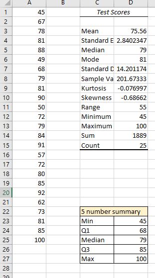
- Obtain the descriptive statistics. What are the mean, median, and mode? What is the standard deviation? Does the data appear to be tightly centered or more spread out? What is the skewness? Does the mean appear to have been pulled left or right of center by any extra large or extra small values?
- Now create a frequency table and histogram. Use class intervals that correspond with letter grades: [latex]40-59[/latex], [latex]60-69[/latex], and so on.

Step [latex]2[/latex]: Create a five-number summary
You may recall from a previous section in the text that a five-number summary is a way of summarizing quantitative data using quartiles.
Quartiles
Quartiles are values that divide the data in quarters.
The first quartile (Q[latex]1[/latex]) is the value so that [latex]25%[/latex] of the data values are below it; the third quartile (Q[latex]3[/latex]) is the value so that [latex]75%[/latex] of the data values are below it. You may have guessed that the second quartile is the same as the median, since the median is the value so that [latex]50%[/latex] of the data values are below it.
This divides the data into quarters; [latex]25%[/latex] of the data is between the minimum and Q[latex]1[/latex], [latex]25%[/latex] is between Q[latex]1[/latex] and the median, [latex]25%[/latex] is between the median and Q[latex]3[/latex], and [latex]25%[/latex] is between Q[latex]3[/latex] and the maximum value.
Five-Number Summary
The five-number summary takes this form:
Minimum, Q[latex]1[/latex], Median, Q[latex]3[/latex], Maximum
Taking Care in the Details
The real power of using a spreadsheet isn’t revealed the first time you use it to run an analysis or computation for you. Designing and creating a spreadsheet often takes longer than just doing the calculation by hand. The real power is revealed in using the sheet repeatedly. A few tedious long moments spent storing functions and formulas and testing them carefully can free up precious time in the future. As you type the formulas in, practice being careful and accurate.
Excel can find the five-number summary for us.
- Type the label “five-number summary” into cell C22.
- Type the words Min, Q[latex]1[/latex], Median, Q[latex]3[/latex], and Max into cells C23, C24, C25, C26, and C27, respectively.
- We are going to use Excel’s QUARTILE.INC() function to find the [latex]5[/latex] numbers. The formula takes as its input, the data list, followed by a comma, followed by a quantity. The quantity for the Min is [latex]0[/latex]. For Q[latex]1[/latex], it’s [latex]1[/latex]. For the Median, it’s [latex]2[/latex]. For Q[latex]3[/latex], it’s [latex]3[/latex]. And for the Max, it’s [latex]4[/latex]. You could also use the MIN() and MAX() functions to get those numbers. The array of data is A1:A25.
- Into cell D23, type =QUARTILE.INC(A1:A25,[latex]0[/latex]) and enter. Notice that the cell is populated with the minimum data element, [latex]45[/latex].
- Into cell D24, type =QUARTILE.INC(A1:A25,[latex]1[/latex])
- Into cell D25, type =QUARTILE.INC(A1:A25,[latex]2[/latex])
- Into cell D26, type =QUARTILE.INC(A1:A25,[latex]3[/latex])
- Into cell D26, type =QUARTILE.INC(A1:A25,[latex]4[/latex])
- Highlight the data in A1 – A25 then click Insert. Under charts, look for the icon that resembles a histogram, Statistical Charts, and click it. Then choose Box and Whisker and click it.
- Note the box plot is vertical. You can change the Chart Title or delete it. The horizontal axis is labeled “[latex]1[/latex]” because we just have [latex]1[/latex] data series in the graph. You can delete that or change it. If you right-click on the blue box then choose data labels, you’ll see the five-number summary show up in the graph.
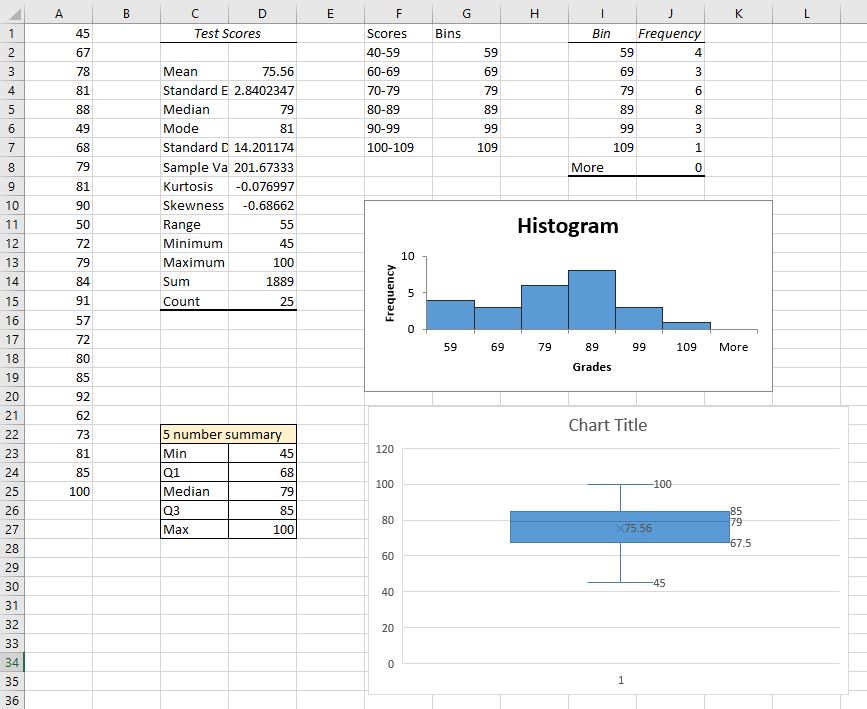
Step [latex]3[/latex]: Analyze the data representations
Analyzing the graphical representation of the data, we can see that, even though several students did well on the test, the mean seems to have been pulled to the left of center by the [latex]4[/latex] failing scores. The teacher can use all of these representations — the list of scores, the table, and the graphs — to make decisions about possible adjustments to her learning environment.