- Find the average, middle value, and most common value in a set of data
- Calculate how spread out the data is using the range and standard deviation
- Identify the parts of a five-number summary for a set of data and create a box plot
Mean, Median, and Mode
The Main Idea
Mean, median, and mode are three types of statistical measures used to analyze a set of data.
The mean, often referred to as the “average,” is calculated by adding all the numbers in a data set and then dividing by the count of those numbers.
[latex]\text{mean}={\Large\frac{\text{sum of values in data set}}{n}}[/latex]
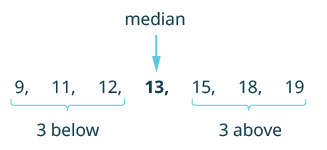
The median is the middle number when the data set is arranged in ascending or descending order; if the data set has an even number of observations, the median is the average of the two middle numbers.
The mode, on the other hand, is the number that occurs most frequently in a data set.
You can view the transcript for “Math Antics – Mean, Median and Mode” here (opens in new window).
Find her median score.

The ages of the students in a statistics class are listed here:
[latex]19[/latex] , [latex]20[/latex] , [latex]23[/latex] , [latex]23[/latex] , [latex]38[/latex] , [latex]21[/latex] , [latex]19[/latex] , [latex]21[/latex] , [latex]19[/latex] , [latex]21[/latex] , [latex]20[/latex] , [latex]43[/latex] , [latex]20[/latex] , [latex]23[/latex] , [latex]17[/latex] , [latex]21[/latex] , [latex]21[/latex] , [latex]20[/latex] , [latex]29[/latex] , [latex]18[/latex] , [latex]28[/latex].
What is the mode?
Students listed the number of members in their household as follows:
[latex]6[/latex] , [latex]2[/latex] , [latex]5[/latex] , [latex]6[/latex] , [latex]3[/latex] , [latex]7[/latex] , [latex]5[/latex] , [latex]6[/latex] , [latex]5[/latex] , [latex]3[/latex] , [latex]4[/latex] , [latex]4[/latex] , [latex]5[/latex] , [latex]7[/latex] , [latex]6[/latex] , [latex]4[/latex] , [latex]5[/latex] , [latex]2[/latex] , [latex]1[/latex] , [latex]5[/latex].
What is the mode?
Range, Standard Deviation, and Variance
The Main Idea
Range, standard deviation, and variance are three key measures of dispersion in a dataset.
The range of a dataset is the difference between the highest and lowest values, giving a simple measure of total spread.
[latex]\text{Range } = \text{ maximum value } – \text{ minimum value } = \text{ largest value } – \text{ smallest value}[/latex]
Standard deviation, a more complex measure, gauges the amount of variation or dispersion of a set of values. A low standard deviation indicates that the values are close to the mean, while a high standard deviation suggests greater dispersion.
A few important characteristics:
- Standard deviation is always positive. Standard deviation will be zero if all the data values are equal, and will get larger as the data spreads out.
- Standard deviation has the same units as the original data.
- Standard deviation, like the mean, can be highly influenced by outliers.
The following formulas are used to calculate the standard deviation of a population and a sample:
Standard deviation of a population: [latex]\sigma = \sqrt{\dfrac{\sum \left(x-\mu\right)^2}{n}}[/latex], where [latex]\mu[/latex] represents the population mean.
Standard deviation of a sample: [latex]s=\sqrt{\dfrac{\sum \left(x-\bar{x}\right)^2}{n-1}}[/latex], where [latex]\bar{x}[/latex] represents the sample mean.
Variance, often denoted by the squared units of the original data, is the average of the squared differences from the mean, effectively measuring how far each number in the set is from the mean.
Variance of a population: [latex]\sigma^{2}=\dfrac{\sum\left(x-\mu\right)^{2}}{n}[/latex]
Variance of a sample: [latex]s^{2}=\dfrac{\sum\left(x-\bar{x}\right)^{2}}{n-1}[/latex]
You can view the transcript for “Measures of Variability (Range, Standard Deviation, Variance)” here (opens in new window).
Five-Number Summary
The Main Idea
The Five-Number Summary is a descriptive statistic that provides information about a dataset. It consists of five values: the minimum, the first quartile (Q1 or 25th percentile), the median (or Q2 or 50th percentile), the third quartile (Q3 or 75th percentile), and the maximum. The minimum and maximum values depict the smallest and largest numbers in the dataset respectively. The first quartile is the median of the lower half of the data (not including the overall median), the third quartile is the median of the upper half, and the median is the middle value of the entire dataset.
To find the first quartile, [latex]Q1[/latex]:
- Begin by ordering the data from smallest to largest
- Compute the locator: [latex]L = 0.25n[/latex]
- If [latex]L[/latex] is a decimal value:
- Round up to [latex]L+[/latex]
- Use the data value in the [latex]L+[/latex]th position
- If [latex]L[/latex] is a whole number:
- Find the mean of the data values in the [latex]L[/latex]th and [latex]L+1[/latex]th positions.
To find the third quartile, [latex]Q3[/latex]:
Use the same procedure as for [latex]Q1[/latex], but with locator: [latex]L = 0.75n[/latex]
You can view the transcript for “What is a 5 Number Summary?” here (opens in new window).
Boxplots
The Main Idea
Box plots, also known as box-and-whisker plots, are graphical representations used to depict the spread and skewness of a data set.
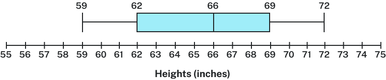
They are constructed using the five-number summary: the minimum, first quartile (Q1), median, third quartile (Q3), and maximum.
The interquartile range (sometimes denoted as IQR) is the difference between the quartiles calculated as
[latex]Q3 – Q1[/latex].
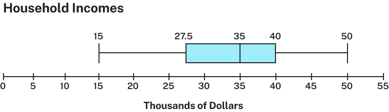
The ‘box’ of the plot represents the interquartile range (IQR), stretching from Q1 to Q3, and the line inside the box marks the median. ‘Whiskers’ extend from the box to the minimum and maximum values, showing the full spread of the data. Outliers, if any, are typically indicated as individual points beyond the whiskers.
You can view the transcript for “BOX AND WHISKER PLOTS EXPLAINED!” here (opens in new window).
The box plot below is based on the household income data with five-number summary: