Exponential and Logarithmic Equations: Get Stronger Key
Logarithmic Properties
3. [latex]{\mathrm{log}}_{b}\left(2\right)+{\mathrm{log}}_{b}\left(7\right)+{\mathrm{log}}_{b}\left(x\right)+{\mathrm{log}}_{b}\left(y\right)[/latex]
5. [latex]{\mathrm{log}}_{b}\left(13\right)-{\mathrm{log}}_{b}\left(17\right)[/latex]
7. [latex]-k\mathrm{ln}\left(4\right)[/latex]
9. [latex]\mathrm{ln}\left(7xy\right)[/latex]
11. [latex]{\mathrm{log}}_{b}\left(4\right)[/latex]
13. [latex]{\text{log}}_{b}\left(7\right)[/latex]
15. [latex]15\mathrm{log}\left(x\right)+13\mathrm{log}\left(y\right)-19\mathrm{log}\left(z\right)[/latex]
17. [latex]\frac{3}{2}\mathrm{log}\left(x\right)-2\mathrm{log}\left(y\right)[/latex]
19. [latex]\frac{8}{3}\mathrm{log}\left(x\right)+\frac{14}{3}\mathrm{log}\left(y\right)[/latex]
21. [latex]\mathrm{ln}\left(2{x}^{7}\right)[/latex]
23. [latex]\mathrm{log}\left(\frac{x{z}^{3}}{\sqrt{y}}\right)[/latex]
27. [latex]{\mathrm{log}}_{11}\left(5\right)=\frac{{\mathrm{log}}_{5}\left(5\right)}{{\mathrm{log}}_{5}\left(11\right)}=\frac{1}{b}[/latex]
29. [latex]{\mathrm{log}}_{11}\left(\frac{6}{11}\right)=\frac{{\mathrm{log}}_{5}\left(\frac{6}{11}\right)}{{\mathrm{log}}_{5}\left(11\right)}=\frac{{\mathrm{log}}_{5}\left(6\right)-{\mathrm{log}}_{5}\left(11\right)}{{\mathrm{log}}_{5}\left(11\right)}=\frac{a-b}{b}=\frac{a}{b}-1[/latex]
31. 3
33. 2.81359
35. 0.93913
37. –2.23266
39. x = 4; By the quotient rule: [latex]{\mathrm{log}}_{6}\left(x+2\right)-{\mathrm{log}}_{6}\left(x - 3\right)={\mathrm{log}}_{6}\left(\frac{x+2}{x - 3}\right)=1[/latex].
Rewriting as an exponential equation and solving for x:
[latex]\begin{cases}{6}^{1}\hfill & =\frac{x+2}{x - 3}\hfill \\ 0\hfill & =\frac{x+2}{x - 3}-6\hfill \\ 0\hfill & =\frac{x+2}{x - 3}-\frac{6\left(x - 3\right)}{\left(x - 3\right)}\hfill \\ 0\hfill & =\frac{x+2 - 6x+18}{x - 3}\hfill \\ 0\hfill & =\frac{x - 4}{x - 3}\hfill \\ \text{ }x\hfill & =4\hfill \end{cases}[/latex]
Checking, we find that [latex]{\mathrm{log}}_{6}\left(4+2\right)-{\mathrm{log}}_{6}\left(4 - 3\right)={\mathrm{log}}_{6}\left(6\right)-{\mathrm{log}}_{6}\left(1\right)[/latex] is defined, so x = 4.
Exponential and Logarithmic Equations
2. An extraneous solution occurs when solving the equation results in a value that does not satisfy the original equation. It can be recognized by substituting the solution back into the original equation and seeing that it makes the equation false or violates a domain restriction (for example, giving a negative input to a logarithm or an even root, or causing division by zero).
3. The one-to-one property can be used if both sides of the equation can be rewritten as a single logarithm with the same base. If so, the arguments can be set equal to each other, and the resulting equation can be solved algebraically. The one-to-one property cannot be used when each side of the equation cannot be rewritten as a single logarithm with the same base.
5. [latex]x=-\frac{1}{3}[/latex]
7. n = –1
9. [latex]b=\frac{6}{5}[/latex]
11. x = 10
13. No solution
15. [latex]p=\mathrm{log}\left(\frac{17}{8}\right)-7[/latex]
21. [latex]x=\mathrm{ln}12[/latex]
27. [latex]x=\mathrm{ln}\left(3\right)[/latex]
31. n = 49
33. [latex]k=\frac{1}{36}[/latex]
35. [latex]x=\frac{9-e}{8}[/latex]
37. n = 1
39. No solution
41. No solution
43. [latex]x=\pm \frac{10}{3}[/latex]
51. x = 9
53. [latex]x=\frac{{e}^{2}}{3}\approx 2.5[/latex]
55. x = –5
57. [latex]x=\frac{e+10}{4}\approx 3.2[/latex]
59. No solution
61. [latex]x=\frac{11}{5}\approx 2.2[/latex]
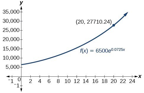
65. about $27,710.24
67. about 5 years
69. [latex]\frac{\mathrm{ln}\left(17\right)}{5}\approx 0.567[/latex]
71. [latex]x=\frac{\mathrm{log}\left(38\right)+5\mathrm{log}\left(3\right)\text{ }}{4\mathrm{log}\left(3\right)}\approx 2.078[/latex]
73. [latex]x\approx 2.2401[/latex]
75. [latex]x\approx -44655.7143[/latex]
77. about 5.83
81. [latex]t=\mathrm{ln}\left({\left(\frac{T-{T}_{s}}{{T}_{0}-{T}_{s}}\right)}^{-\frac{1}{k}}\right)[/latex]
Exponential and Logarithmic Models
1. Half-life is a measure of decay and is thus associated with exponential decay models. The half-life of a substance or quantity is the amount of time it takes for half of the initial amount of that substance or quantity to decay.
7. [latex]f\left(0\right)\approx 16.7[/latex]; The amount initially present is about 16.7 units.
9. 150
11. exponential; [latex]f\left(x\right)={1.2}^{x}[/latex]
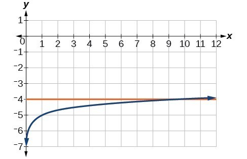
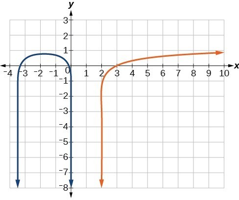
13. logarithmic
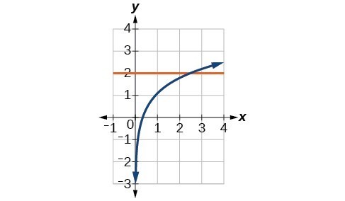
15. logarithmic
17.
21. about 7.3 years
23. 4 half-lives; 8.18 minutes
25. [latex]\begin{cases}\text{ }M=\frac{2}{3}\mathrm{log}\left(\frac{S}{{S}_{0}}\right)\hfill \\ \mathrm{log}\left(\frac{S}{{S}_{0}}\right)=\frac{3}{2}M\hfill \\ \text{ }\frac{S}{{S}_{0}}={10}^{\frac{3M}{2}}\hfill \\ \text{ }S={S}_{0}{10}^{\frac{3M}{2}}\hfill \end{cases}//[/latex]
28. 2 hours.
29. [latex]A=125{e}^{\left(-0.3567t\right)};A\approx 43[/latex] mg
31. about 60 days
32. [latex]A(t)=0.5(0.9885)^t[/latex]. After 60 days, [latex]A(60)\approx 0.3[/latex] grams.
33. [latex]f\left(t\right)=250{e}^{\left(-0.00914t\right)}[/latex]; half-life: about [latex]\text{76}[/latex] minutes
35. [latex]r\approx -0.0667[/latex], So the hourly decay rate is about 6.67%
37. [latex]f\left(t\right)=1350{e}^{\left(0.03466t\right)}[/latex]; after 3 hours: [latex]P\left(180\right)\approx 691,200[/latex]
40. [latex]T(t)=69+31e^{\left(\frac{1}{15}\ln\left(\frac{26}{31}\right)\right)t}[/latex].
41. about 88 minutes
Fitting Exponential Models to Data
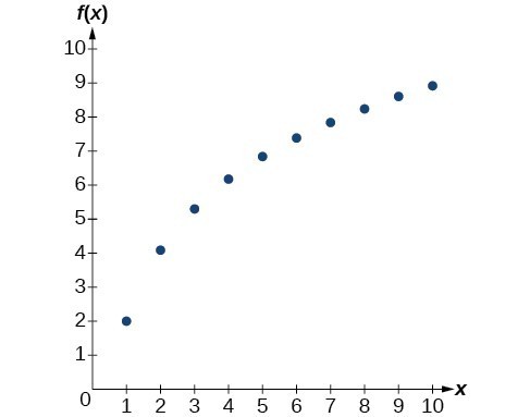
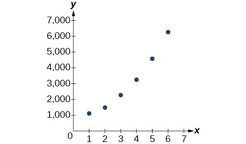
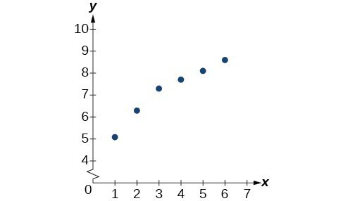
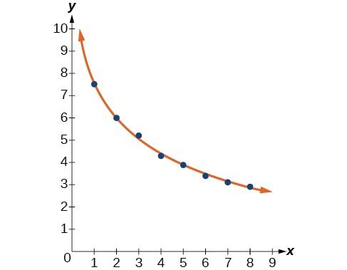
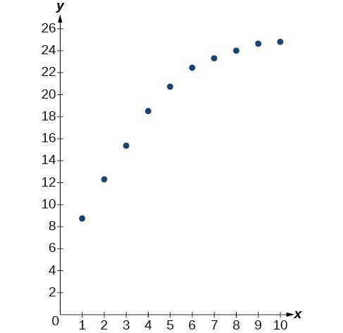
4. A scatterplot that is best described by a logarithmic model would show a rapid increase or decrease at first, followed by a gradual leveling off as the input values increase. The data points would form a curve that rises (or falls) quickly and then flattens.
6. E
7. C
8. A
9. B
10. D
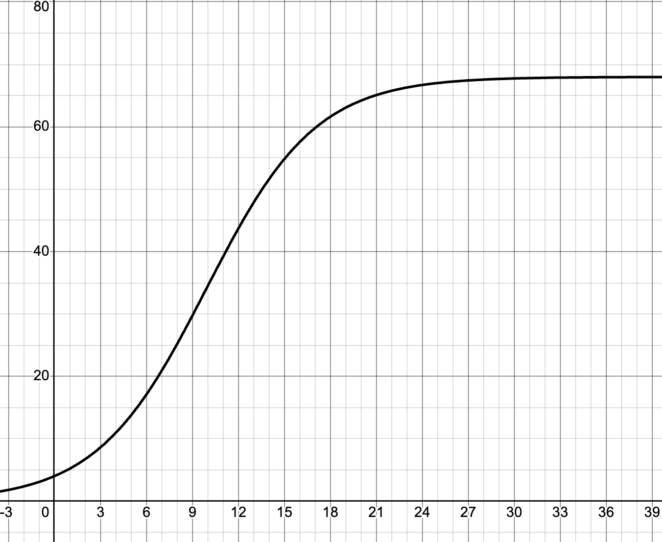
11. [latex]P\left(0\right)=22[/latex] ; 175
13. [latex]p\approx 2.67[/latex]
16. 
17. 4 koi
18. 6.8 months
20. 
21. 10 wolves
23. about 5.4 years.
25.
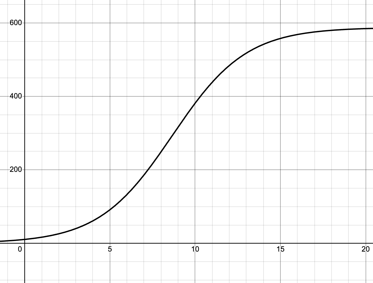
26. [latex]f(x)\approx 795(1.415)^x[/latex]
31. [latex]f\left(x\right)=731.92{\left(0.738\right)}^{x}[/latex]
35.
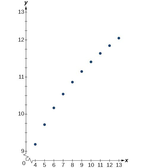
36. [latex]y\approx 5.06+1.93\ln(x)[/latex]
37. [latex]f\left(10\right)\approx 9.5[/latex]
40. 
41. [latex]f\left(x\right)=7.544 - 2.268\mathrm{ln}\left(x\right)[/latex]
45.
46. [latex]y\approx 26.91-24.20e^{-0.264x}[/latex]
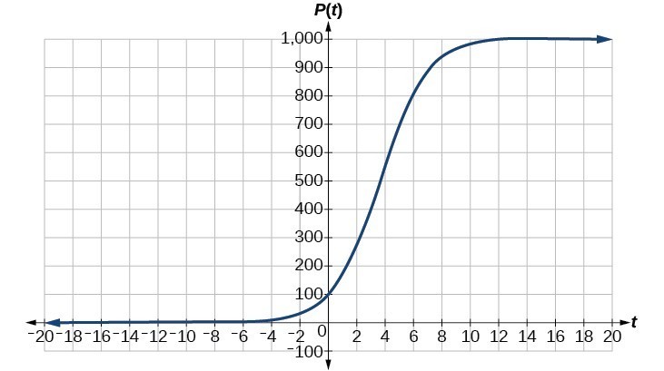
51. [latex]f\left(x\right)=\frac{136.068}{1+10.324{e}^{-0.480x}}[/latex]
53. about 136