Logarithmic Properties
- [latex]\log_b(2)+\log_b(7)+\log_b(x)+\log_b(y)[/latex]
- [latex]\log_b(13)-\log_b(17)[/latex]
- [latex]-k\ln(4)[/latex]
- [latex]\ln(7xy)[/latex]
- [latex]\log_b(4)[/latex]
- [latex]\log_b(7)[/latex]
- [latex]15\log(x)+13\log(y)-19\log(z)[/latex]
- [latex]\dfrac{3}{2}\log(x)-2\log(y)[/latex]
- [latex]\dfrac{8}{3}\log(x)+\dfrac{14}{3}\log(y)[/latex]
- [latex]\ln(2x^7)[/latex]
- [latex]\log(\dfrac{xz^3}{\sqrt{y}})[/latex]
- [latex]\log_7(15)=\dfrac{\ln(15)}{\ln(7)}[/latex]
- [latex]\log_{11}(5)=\dfrac{\log_5(5)}{\log_5(11)}=\dfrac{1}{b}[/latex]
- [latex]\log_{11}(\dfrac{6}{11})=\dfrac{\log_5(\dfrac{6}{11})}{\log_5(11)}=\dfrac{\log_5(6)-\log_5(11)}{\log_5(11)}=\dfrac{a-b}{b}=\dfrac{a}{b}-1[/latex]
- [latex]3[/latex]
- [latex]2.81359[/latex]
- [latex]0.93913[/latex]
- [latex]-2.23266[/latex]
Exponential and Logarithmic Equations and Models
- [latex]x=-\dfrac{1}{3}[/latex]
- [latex]n=-1[/latex]
- [latex]b=\dfrac{6}{5}[/latex]
- [latex]x=10[/latex]
- No solution
- [latex]p=\log(\dfrac{17}{8})-7[/latex]
- [latex]k=-\dfrac{\ln(38)}{3}[/latex]
- [latex]x=\dfrac{\ln(\dfrac{38}{3})-8}{9}[/latex]
- [latex]x=\ln(12)[/latex]
- [latex]10^{-2}=\dfrac{1}{100}[/latex]
- [latex]n=49[/latex]
- [latex]k=\dfrac{1}{36}[/latex]
- [latex]x=\dfrac{9-e}{8}[/latex]
- [latex]n=1[/latex]
- No solution
- No solution
- [latex]x=\pm\dfrac{10}{3}[/latex]
- [latex]x=10[/latex]
- [latex]x=0[/latex]
- [latex]x=\dfrac{3}{4}[/latex]
Exponential and Logarithmic Models
- [latex]f(0)\approx 16.7[/latex]; The amount initially present is about [latex]16.7[/latex] units.
- [latex]150[/latex]
- exponential; [latex]f(x)=1.2^x[/latex]
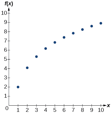
- logarithmic
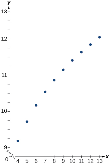
- logarithmic
- about [latex]1.4[/latex] years
- about [latex]7.3[/latex] years
- [latex]A=125e^{(-0.3567t)}[/latex]; [latex]A\approx 43[/latex] mg
- about [latex]60[/latex] days
- [latex]A(t)=250e^{(-0.00822t)}[/latex]; half-life: about [latex]84[/latex] minutes
- [latex]r\approx -0.0667[/latex], So the hourly decay rate is about [latex]6.67 \%[/latex]
- [latex]f(t)=1350e^{(0.03466t)}[/latex]; after [latex]3[/latex] hours: [latex]P(180)\approx 691,200[/latex]
- [latex]f(t)=256e^{(0.068110t)}[/latex]; doubling time: about [latex]10[/latex] minutes
- about [latex]88[/latex] minutes
- [latex]T(t)=90e^{(-0.008377t)}+75[/latex], where [latex]t[/latex] is in minutes.
- about [latex]113[/latex] minutes