• Check the conditions for a [latex]t[/latex]-distribution, then use a [latex]t[/latex]-distribution to calculate probabilities when appropriate.

[latex]t[/latex]-model

On the previous page, we had to supply the population mean, [latex]\mu[/latex], and the population standard deviation, [latex]\sigma[/latex], to calculate the mean and standard deviation of the sample mean, to be used to calculate probabilities. It may have occurred to you that we might not have the population data. If we do not know [latex]\mu[/latex], it is unlikely that we know [latex]\sigma[/latex]. So, we now have to take a different approach. We estimate [latex]\sigma[/latex] using the sample standard deviation, [latex]s[/latex].

The standard error for the sampling distribution [latex]\dfrac{\sigma}{\sqrt{n}}[/latex] becomes [latex]\dfrac{s}{\sqrt{n}}[/latex].

This estimate for [latex]\sigma[/latex] introduces more uncertainty in the process. The problem is worse with smaller samples because the sample standard deviations vary more. For small samples, [latex]s[/latex] is a worse approximation for [latex]\sigma[/latex] . Unfortunately, this approximation makes the normal model a bad fit and inappropriate for determining critical values. We instead use what is called a t-model for this purpose.

Here is the formula for the [latex]t[/latex]-score. We also include the [latex]z[/latex]-score for comparison. 

[latex]z=\dfrac{\stackrel{¯}{x}-μ}{\frac{σ}{\sqrt{n}}}   \rightarrow   t=\dfrac{\stackrel{¯}{x}-μ}{\frac{s}{\sqrt{n}}}[/latex]

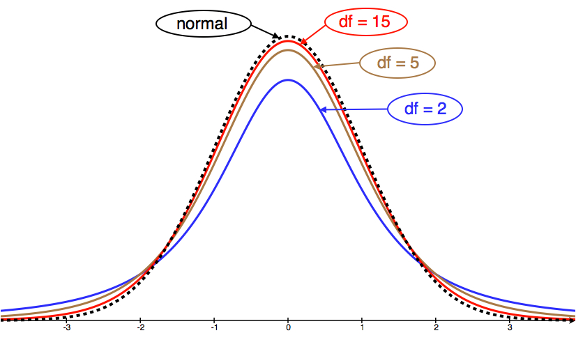
The distribution of [latex]z[/latex]-scores is the standard normal curve, with a mean of 0 and a standard deviation of 1. The distribution of [latex]t[/latex]-scores depends on the sample size, [latex]n[/latex]. There is a different [latex]t[/latex]-model for every [latex]n[/latex]. So the [latex]t[/latex]-model is a family of curves. Instead of referring to [latex]n[/latex] to specify which [latex]t[/latex]-model to use, we refer to the degrees of freedom, or [latex]df[/latex] for short. The number of degrees of freedom is 1 less than the sample size. That is, [latex]df = n – 1[/latex].

[latex]t[/latex]-statistic

When we estimate [latex]\sigma[/latex] using the sample standard deviation, [latex]s[/latex], we use the [latex]t[/latex]–statistic:

 

[latex]t=\dfrac{\bar{x}-[\text{mean of } \bar{x}'s]}{\text{std. error of } \bar{x}'s}[/latex] [latex]= \dfrac{\bar{x}-\mu}{\frac{s}{\sqrt{n}}}[/latex]

 

with a degree of freedom [latex]df = n – 1[/latex].

Let’s take a look at a few [latex]t[/latex]-model curves (for various [latex]df[/latex]) to see how they compare to the normal model.