• Understand the concept of a probability distribution and its role in describing the behavior of a random variable.
• Describe the characteristics of probability distributions.

Continuous Probability Distributions

So far, we have been using a discrete probability distribution that gives the probabilities for a fixed set of values. The spinner can land on purple [latex]2[/latex] or [latex]3[/latex] times, but [latex]2.5[/latex] is impossible. It is not in the set of possible values.

However, some variables are continuous, which means the range of values includes an infinite number of possible values. Consider a person’s height. Although we often measure heights to the nearest inch, a person does not grow in one-inch spurts but instead moves through the range of heights via immeasurably small increments. It is not possible to count all the possible heights that a person can be because even between [latex]64[/latex] inches and [latex]65[/latex] inches, there are infinitely many possible heights.

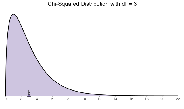
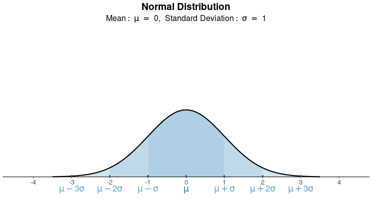
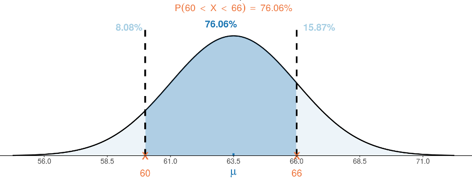
When we are using a discrete probability distribution, we calculate the probability for a range of values by adding up the probability of each outcome in the range. However, when we are using a continuous probability distribution, probabilities are represented as the area under a density curve. The total area under the curve is equal to [latex]1[/latex].

continuous probability distribution

A continuous probability distribution is a probability distribution for a continuous random variable (an infinite and uncountable random variable).

 

The probabilities of a continuous probability distribution are represented as the area under a density curve. The total area under the curve is equal to [latex]1[/latex].

 

Suppose the following graph shows the distribution of heights (in inches) for women in a particular country. To find the probability that a randomly selected woman is between 60 and 66 inches tall, we would shade the area under the curve between these two values.

In some situations, we may use a continuous probability distribution as an approximation even when the variable is technically discrete.