- Recognize when a linear regression model will fit a given data set.
- Use technology to create scatterplots, find the line of best fit, and find the correlation coefficient.
- Find the estimated slope and [latex]y[/latex]-intercept for a linear regression model.
- Use the line of best fit to predict values.
Line of Best Fit
A method we will use to make predictions about missing observations or future observations in bivariate data is called Least Squares Regression (LSR) analysis. The language might seem intimidating at first, but the ideas are quite straightforward, especially with examples to illustrate each new term. For example, LSR analysis can also be described as linear modeling, where we determine the equation of a line of best fit to make predictions based on an existing data set.
line of best fit
The line of best fit is simply the best line that describes the data points. For real data with natural deviations, the line cannot go through all of the points. In fact, very often, the line does not go through any of the data points.
Since no line will be perfect, the best we can do is minimize its error. In this course, we will do this by minimizing the sum total of the squared vertical errors from all data points to the line. This is why the line of best fit is also called the Least Squares Regression Line (LSRL).
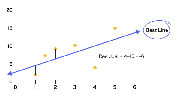
The vertical error associated with each data point is called the residual of that observation. This error, illustrated by the length of the vertical line, represents how far off a prediction calculated from the line is compared to the actual, observed value; the larger the line, the greater the error associated with that particular observation.
Note: For data points that are above the line of best fit, the residuals are positive, and for data points that are below the line, the residuals are negative.
equation for the line of best fit
The equation for the line of best fit is very similar to one you may have seen in a previous math class:
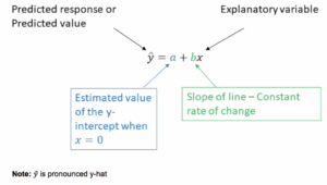
An important distinction between the [latex]y=mx+b[/latex] linear model and the [latex]\displaystyle\hat{{y}}={a}+{b}{x}[/latex] linear model is that in statistics, we are estimating the equation of the line from data. This estimate is denoted by the “hat” symbol (^), which signifies a value estimated by the model rather than a known quantity. Please keep this distinction in mind as we progress through the upcoming activities, where we will be interpreting the estimated or predicted slopes and estimated or predicted intercepts generated from given data sets.
The calculations of the estimated slope and the estimated y-intercept come directly from the data set. Below are the formulas for [latex]a[/latex] and [latex]b[/latex]:
- The estimated [latex]y[/latex]-intercept is [latex]\displaystyle{a}=\overline{y}-{b}\overline{{x}}[/latex].
- Note: The sample means of the [latex]x[/latex] values and the [latex]y[/latex] values are [latex]\displaystyle\overline{{x}}[/latex] and [latex]\overline{{y}}[/latex].
- The estimated slope is [latex]b=r(\frac{{s}_{y}}{{s}_{x}})[/latex].
- Note: [latex]s_y[/latex] represents the standard deviation of the [latex]y[/latex] values (response variable), [latex]s_x[/latex] represents the standard deviation of the [latex]x[/latex] values (explanatory variable), and [latex]r[/latex] is the correlation coefficient.
-
Why are these formulas important?
- They demonstrate that both the estimated slope and intercept are calculated directly from the data. If you change the data, you will almost certainly get a different line of best fit, slope, and intercept.
- The good news is that we will be relying on software for all calculations involved in the line of best fit. However, you will need to use some common sense and appropriate units when providing interpretations.