- Complete a chi-square test for goodness of fit and write its conclusion in context of the problem
Chi-Square ([latex]\chi^2[/latex]) Distribution
Unlike other sampling distributions we have studied, the chi-square model does not have a normal shape. It is skewed to the right. Like the [latex]t[/latex]-model, the chi-square model is a family of curves that depend on degrees of freedom.
- For a chi-square goodness of fit test, the degrees of freedom is (number categories [latex]- 1[/latex]).
- The mean of the chi-square distribution is equal to the degrees of freedom.
conditions for a [latex]\chi^2[/latex] goodness of fit test
A chi-square model is a good fit for the distribution of the chi-square test statistic only if the following conditions are met:
- Random: Observed counts must come from a random sample (to ensure our conclusions are free from sampling bias).
- 10%: The sample size must be less than a tenth of the population size (to satisfy independence assumptions).
- Large Sample: The sample is large enough such that the expected counts are all five or greater (to ensure our sampling distribution resembles a chi-square distribution).
| Sample A |
Quarter 1 (Jan. – March) |
Quarter 2 (April – June) |
Quarter 3 (July – Sept.) |
Quarter 4 (Oct. – Dec.) |
| Observed number of football players | 3 | 4 | 2 | 1 |
| Sample B |
Quarter 1 (Jan. – March) |
Quarter 2 (April – June) |
Quarter 3 (July – Sept.) |
Quarter 4 (Oct. – Dec.) |
| Observed number of football players | 3,000 | 4,000 | 2,000 | 1,000 |
| Sample C |
Quarter 1 (Jan. – March) |
Quarter 2 (April – June) |
Quarter 3 (July – Sept.) |
Quarter 4 (Oct. – Dec.) |
| Observed number of football players | 507 | 534 | 389 | 273 |
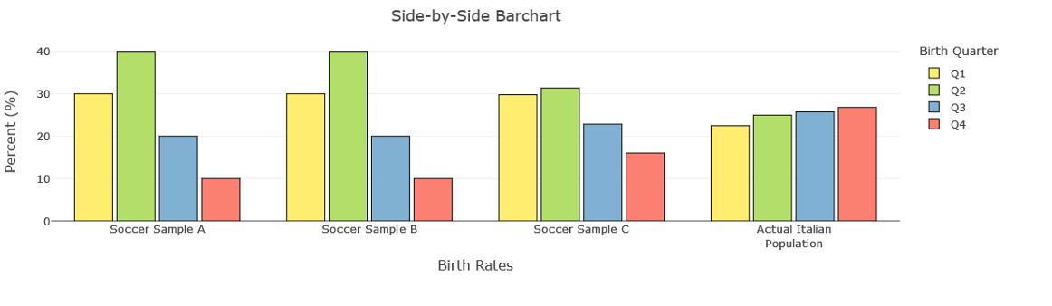
The data in the tables are displayed in the following side-by-side bar chart: