Continuous Random Variables

Previously, we studied discrete (listable) random variables and their distributions. In this section, we will explore continuous (decimal-valued) random variables that can take on values anywhere in an interval. For example, a person’s exact weight without rounding is a continuous random variable. If rounded to the nearest pound, weight is a discrete random variable. Decimal-valued numbers appear frequently in real life, often in measuring things such as weight or length. To best study real-life data, we need to build a solid foundation in continuous probability distributions.

Probability Density Curve

In a continuous probability distribution, probabilities are represented as areas under a curve.

You can see below a histogram of the sodium content in milligrams (mg) of [latex]20[/latex] different cereals modeled by a curve. Note that models are not perfect representations of the data.
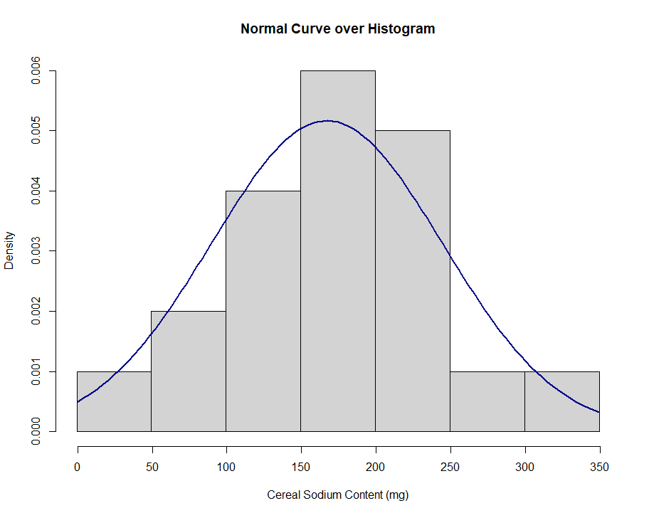
The figure above has a similar shape as the histogram, with a few differences. The y-axis is now labeled “density”.
To understand density, let’s focus on the area in the first bar that represents the cereals with sodium contents between [latex]0[/latex] and [latex]50[/latex] mg. The percentage of cereals that have less than [latex]50[/latex] mg of sodium is [latex]\dfrac{1}{20}[/latex], or [latex]0.05 (5\%)[/latex].

Thus, the shaded area of the density plot that is less than [latex]50[/latex] mg of sodium is [latex]50*0.001 = 0.05[/latex], where [latex]0.001[/latex] is the height of the rectangle and [latex]50[/latex] is the width.