Basic Formatting and Layout: Apply It 1

  • Apply table styles.
  • Apply cell styles.
  • Change cell format.
  • Change comma style.

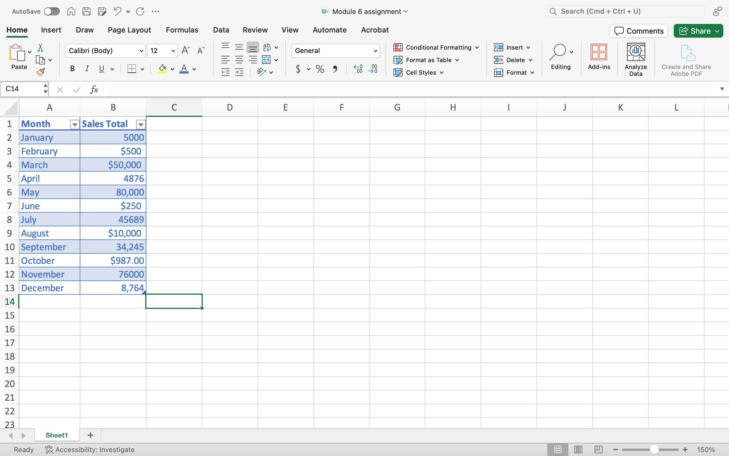
Let’s manipulate an Excel worksheet to organize and display data about sales totals throughout a year.

Download this Excel workbook. It already contains the data you need.

  1. Open the workbook. Save it to the Rowan folder on your desktop as LastName_SalesData.xlsx, replacing “LastName” with your own last name. (Example: Hywater_SalesData) It is a good idea to save your work periodically.
  2. Format the data as a table with the name of the months and sales total as headers. You may use any table style you like.
    A Microsoft Excel sheet is open with content in cells A1 through B13. Cell A is representing months while cell B is representing total sales.
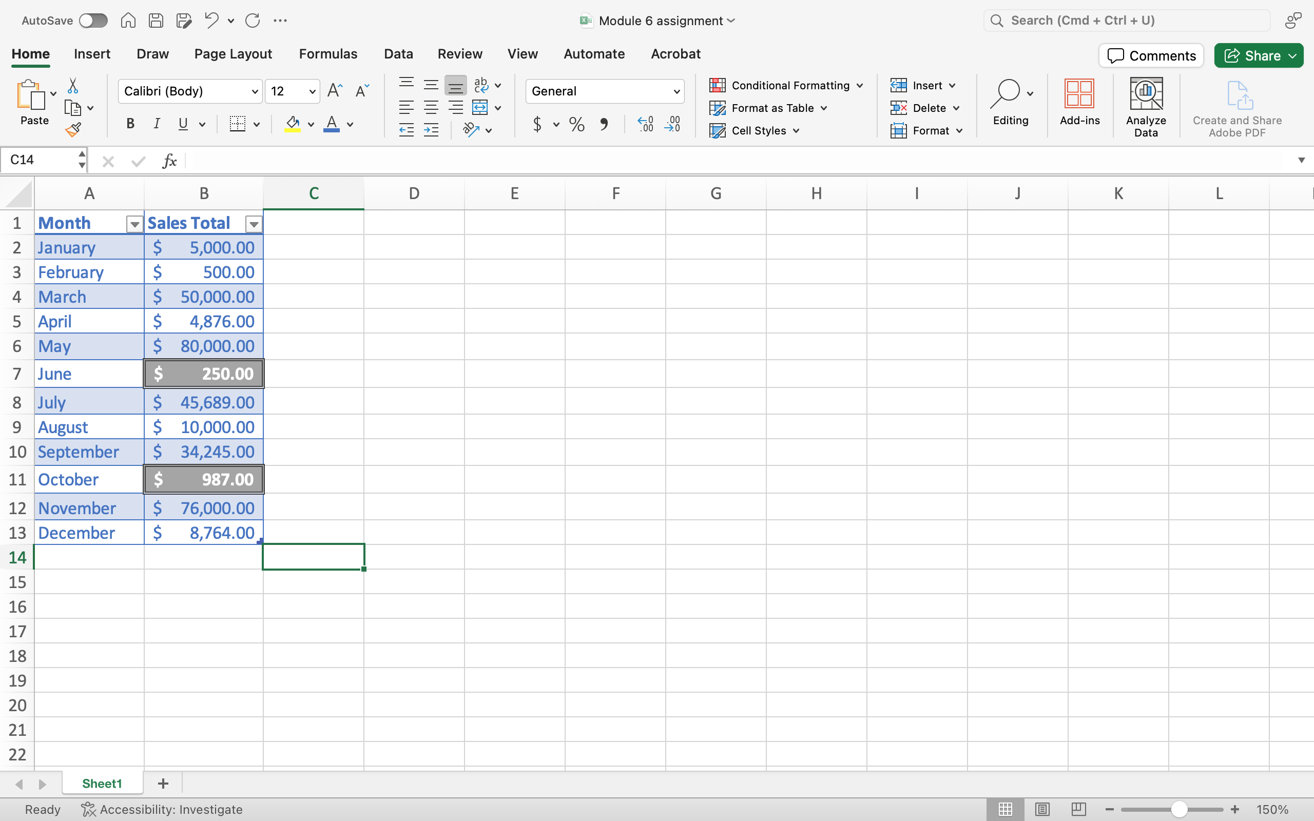
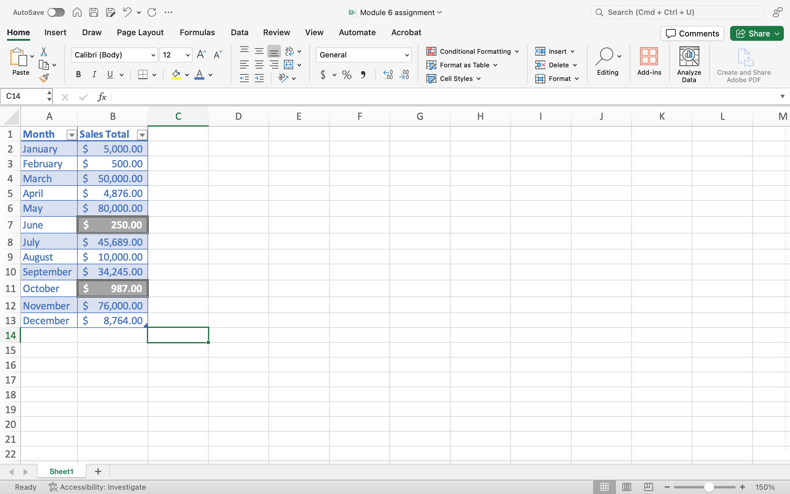
  3. Change the cell format so that all the sales totals display as currency with a dollar sign and two decimal places.
    A Microsoft Excel sheet is open with content in cells A1 through B13. Cell A is representing months while cell B is representing total sales. All of column B has been formatted with dollar signs next to all of the numbers.
  4. Indicate that the data for June and October needs to be verified by applying a different cell style to those cells.
    A Microsoft Excel sheet is open with content in cells A1 through B13. Cell A is representing months while cell B is representing total sales. All of column B has been formatted with dollar signs next to all of the numbers. The data in cells B7 and B11 have been highlighted in gray.
  5. AutoFit the column width.
    A Microsoft Excel sheet is open with content in cells A1 through B13. Cell A is representing months while cell B is representing total sales. All of column B has been formatted with dollar signs next to all of the numbers. The data in cells B7 and B11 have been highlighted in gray. The auto fit column width has been applied.
  6. Save your work! You may need to submit this assignment for your class.