- Use Flash Fill.
- Use AutoSum button.
- Complete simple math functions in Excel
Let’s take a look at the workbook we began last module to analyze trends in sales data over several years.
You will need to download this workbook and open the assignment you completed last module that you saved as LastName_SalesData.xlsx (or you can download the original assignment here)
- Open both workbooks. Save the new file as LastName_YearlyTrends.xlsx, replacing “LastName” with your own last name. (Example: Hywater_YearlyTrends) It is a good idea to save your work periodically.
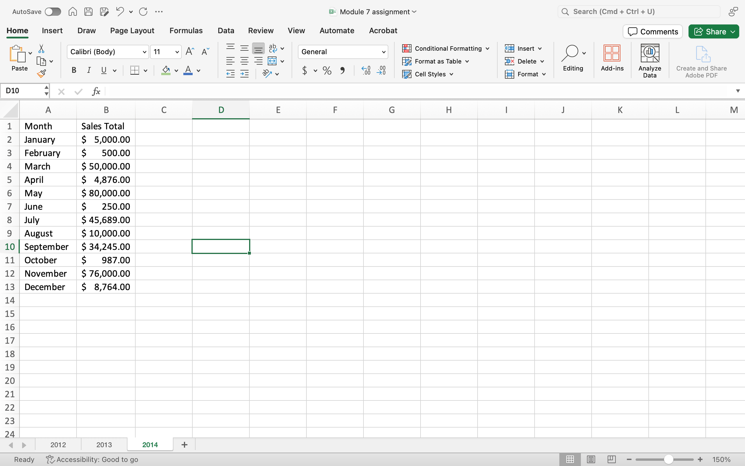
- First, we need to combine the information into a single workbook. Add a new worksheet to the Yearly Trends file and copy the table from the Sales Data assignment to that new tab. Name the new tab “2014.” Be sure to set the number type to currency.
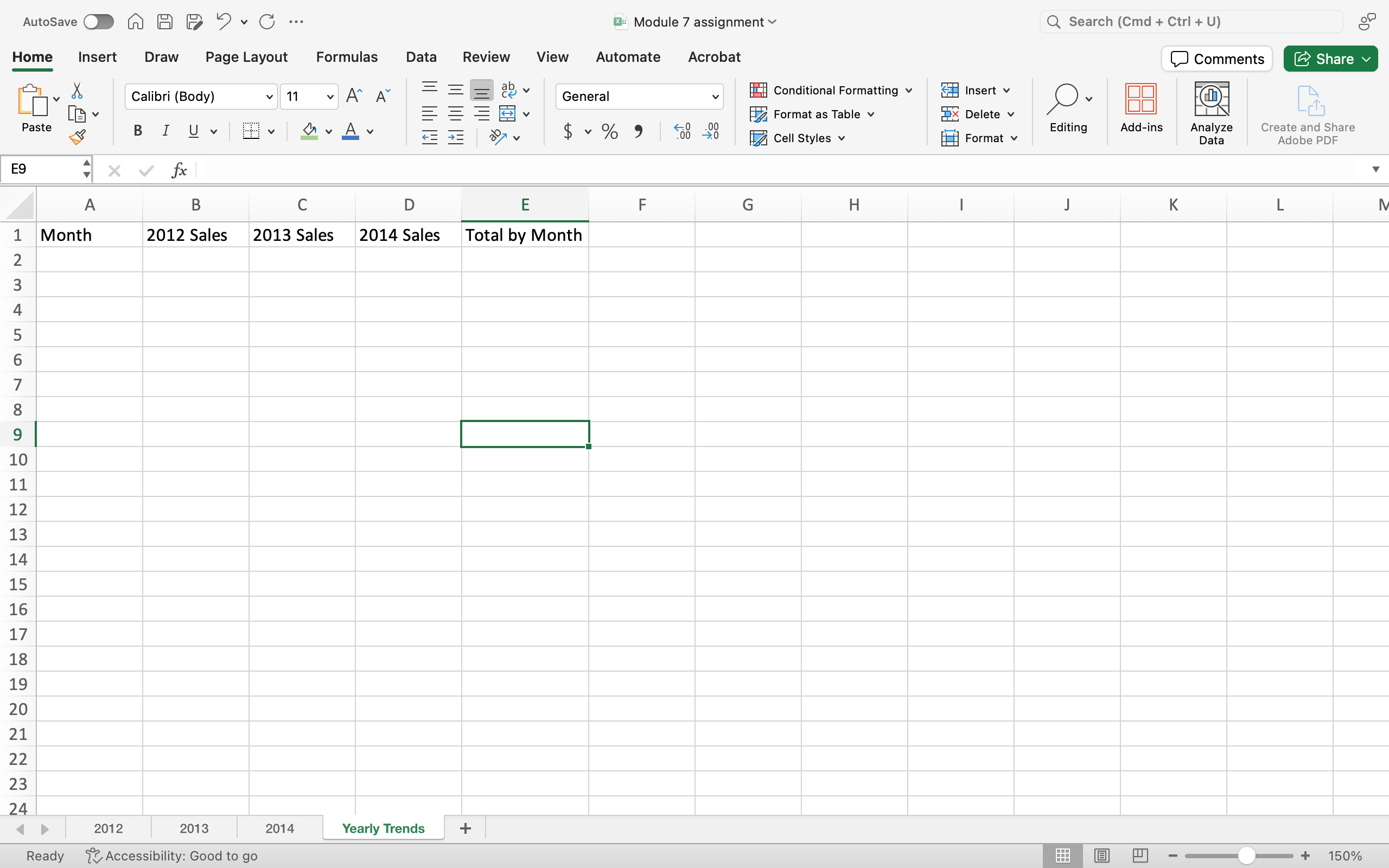
- Add another new worksheet. Now we want to set up the spacing for the table we are about to make. Merge the 1 and 2 cells of column A, B, C, D, and E individually (so A1 and A2 merge, B1 and B2 merge, etc). Then name the cells as shown in the list below and center the text in those cells.
A = Month
B = 2012 Sales
C = 2013 Sales
D = 2014 Sales
E = Total by Month
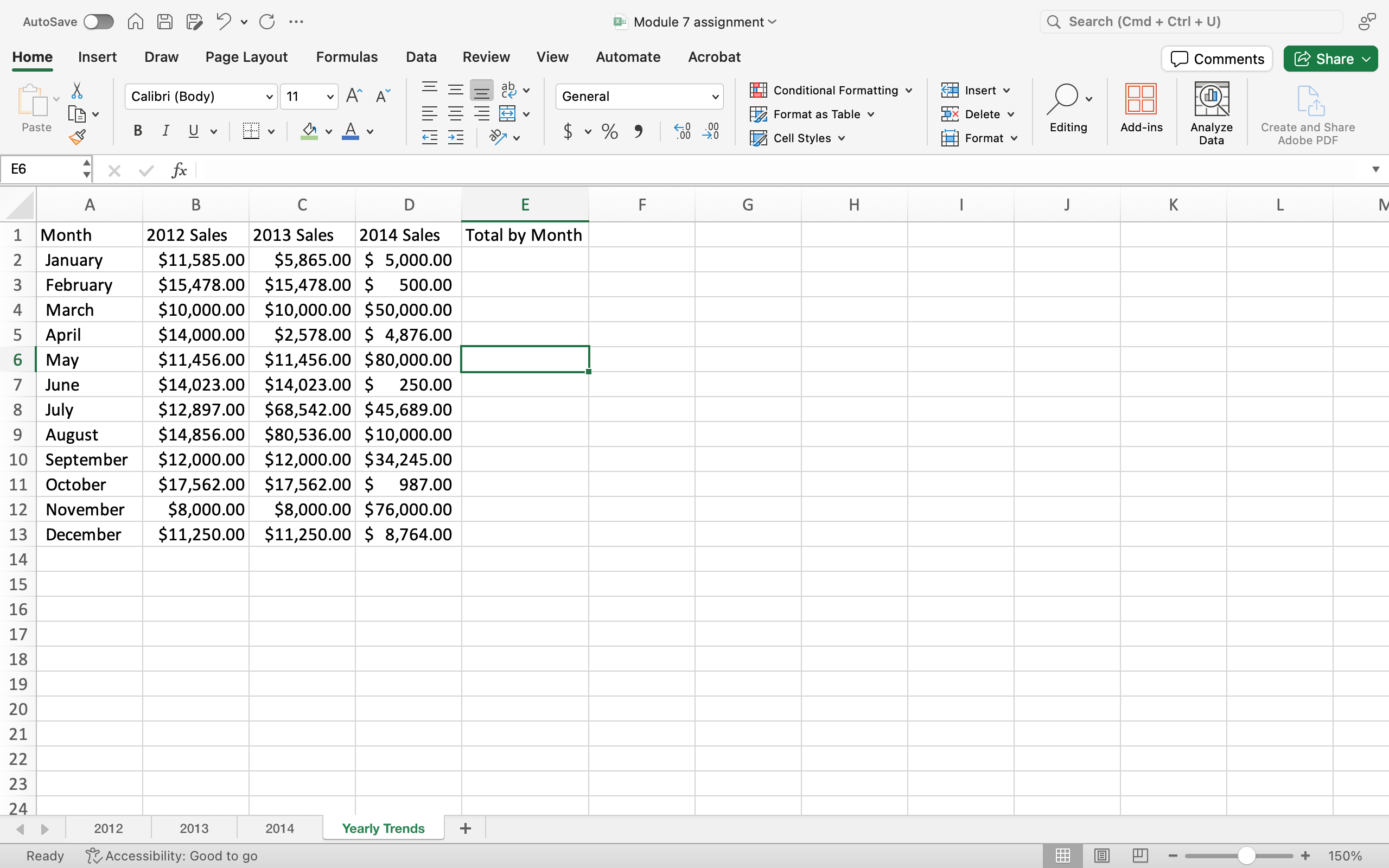
- Copy the following columns of data over in order: “2012 Sales Total,” “2013 Sales Total,” and “2014 Sales Total.” Remember, you can just copy and paste each column in order, using the columns you have already labeled. When you AutoFit the column to the data width, your header cells will change.
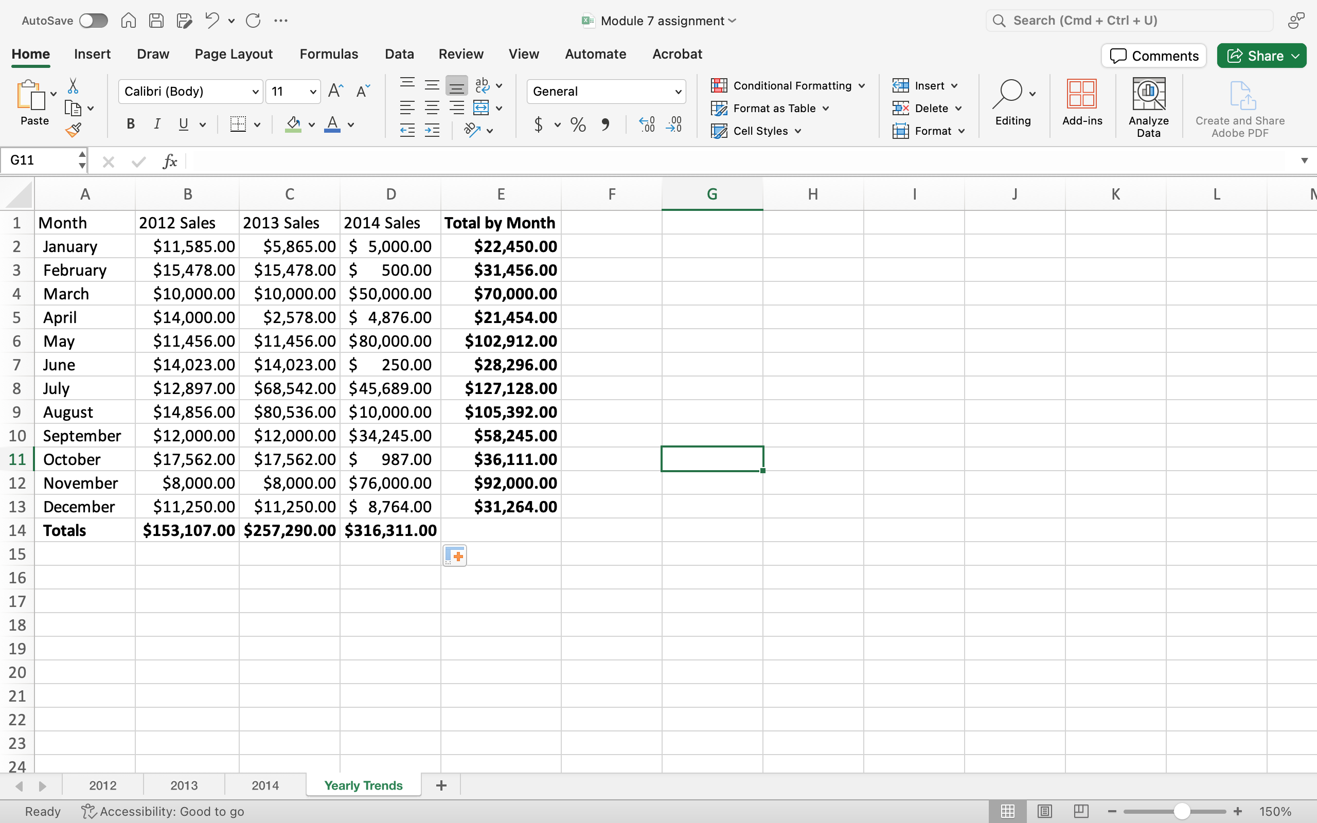
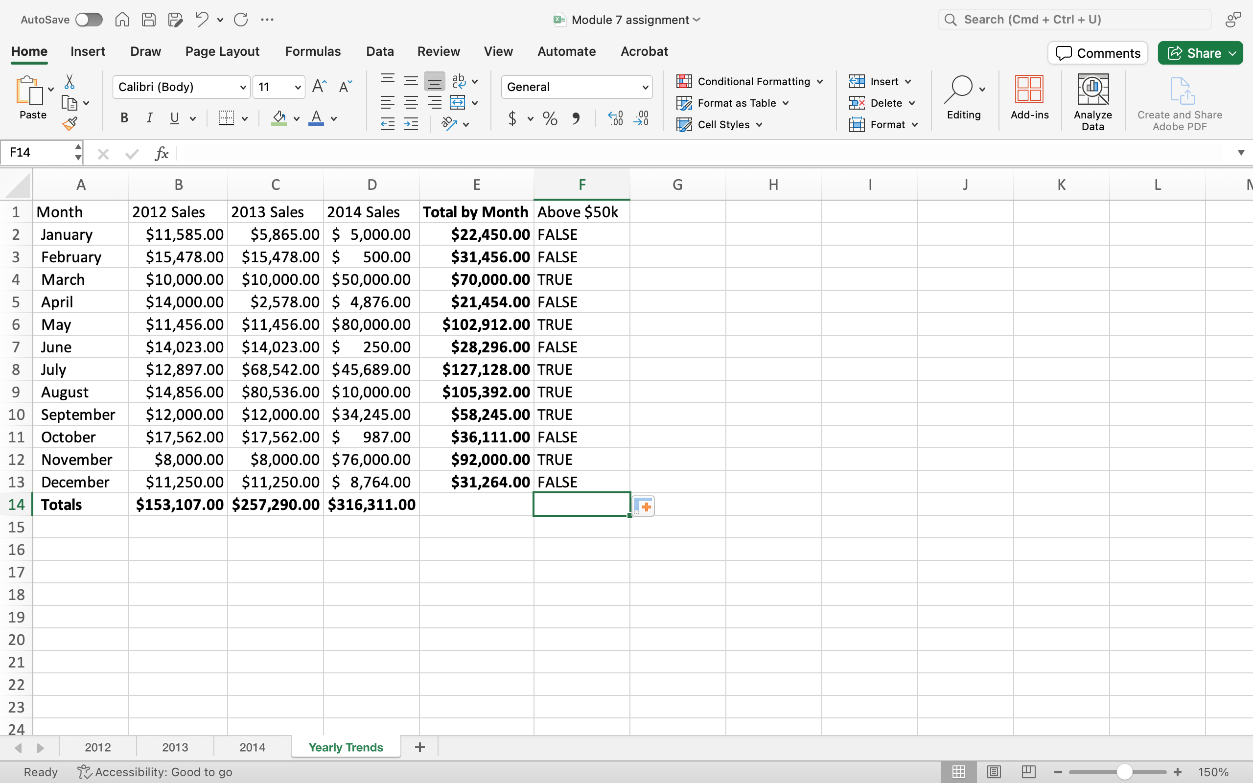
- Now apply Autosum to the sales data for both the total by month and by year. When you have the totals, apply bold to them to make them stand out more and type “Totals” in the cell under December. Autofit the column widths as needed to display all values.
- Merge cells F1 and F2. Next to the ‘Totals by Month’ column, type ‘Above $50k’ in the column title. In the first cell in the new column use an IF function to identify True or False if the totals by month are greater than $50,000 or not. Remember, after you create the first IF functions in January, you can Flash fill the other cells by dragging the bottom right of the highlighted cell down the other cells.
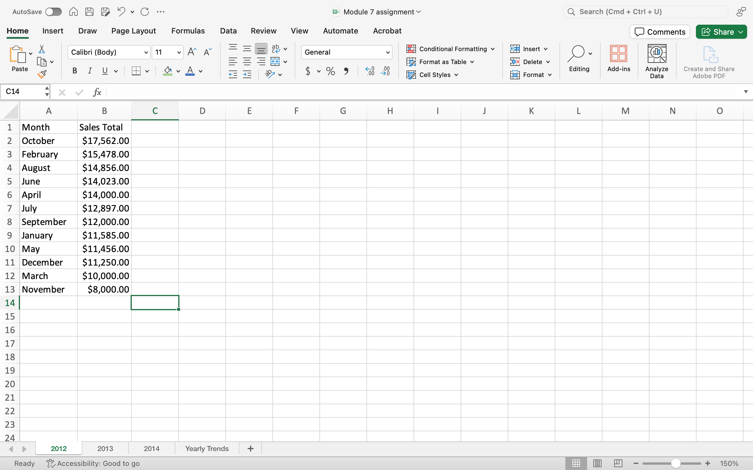
- Return to the individual tabs for each year. For each year of data, sort the sales total “Z to A” so that the month with the highest sales is at the top. When you chose the “Sort” option, be sure to “Expand the Selection.” That will make sure that the months change as well. The screenshot below shows you only what 2012 should look like, but when you finish you should see October as the highest in 2012, August for 2013, and May for 2014.
- Save your work; you may need to submit this online.