- Recognize polynomial functions, noting their degree and leading coefficient
- Apply various methods to divide polynomials and locate the zeros of polynomial equations
- Generate graphs and formulate equations for polynomial functions
- Explain the end behavior of polynomial functions
Identifying Polynomial Functions
The Main Idea
Polynomial functions are like the DNA of algebra—they combine simplicity and complexity to form an incredibly diverse array of functions.
At their core, polynomials are sums of terms made up of coefficients and variables raised to whole number powers. The degree of a polynomial, given by the highest power of the variable, tells us a lot about the function’s behavior and the shape of its graph.
Let [latex]n[/latex] be a non-negative integer. A polynomial function is a function that can be written in the form
[latex]f\left(x\right)={a}_{n}{x}^{n}+\dots+{a}_{2}{x}^{2}+{a}_{1}x+{a}_{0}[/latex]
This is called the general form of a polynomial function.
Each [latex]{a}_{i}[/latex] is a coefficient and can be any real number.
Each product [latex]{a}_{i}{x}^{i}[/latex] is a term of a polynomial function.
Quick Tips
- Linear, Quadratic, and Beyond: A first-degree polynomial is linear, a second-degree is quadratic, and higher degrees have their own characteristics and complexities.
- Coefficient Clues: The coefficients in a polynomial can tell us about the steepness and direction of the graph. A positive leading coefficient means the graph opens upward, and a negative one indicates it opens downward.
Defining the Degree and Leading Coefficient of a Polynomial Function
The Main Idea
The degree of a polynomial is the highest power of the variable present. The leading coefficient is the coefficient of the term with the highest power. These two characteristics can tell us a lot about the function’s behavior, especially its growth and end behavior.
-
Degree Tells the Tale: The degree of a polynomial function hints at the number of roots and the possible number of turns on its graph. For instance, a second-degree polynomial, or a quadratic, will have at most two roots and one turn.
-
Leading Coefficient Impact: The leading coefficient isn’t just a number—it’s the boss. It influences the end behavior of the polynomial’s graph. If it’s positive, the graph eventually rises; if negative, the graph falls.
Quick Tips: Identifying Degree and Leading Coefficient
- Arrange terms in descending order of power to easily identify the leading term and coefficient.
- The degree gives a sense of the ‘shape’ of the graph of the polynomial function.
- For instance, [latex]f(x)=3+2x^2−4x^3[/latex] has a degree of [latex]3[/latex] and a leading coefficient of [latex]-4[/latex], indicating a cubic function with a negative leading term.
Identify the degree, leading term, and leading coefficient of the polynomial [latex]f\left(x\right)=4{x}^{2}-{x}^{6}+2x - 6[/latex].
Watch the following video for more examples of how to determine the degree, leading term, and leading coefficient of a polynomial.
You can view the transcript for “Degree, Leading Term, and Leading Coefficient of a Polynomial Function” here (opens in new window).
Polynomial Long Division
The Main Idea
Polynomial long division might seem daunting at first, but it’s quite similar to the long division we learned in elementary school. Just like we divide numbers, we can divide polynomials, breaking them down into simpler parts. The process involves dividing the highest degree terms and then subtracting to find the remainder, which we then bring down the next term to continue the process.
Quick Tips: Steps to Polynomial Long Division
- Set Up: Write the polynomial (dividend) and the binomial (divisor) in long division format.
- Divide the Leading Terms: Take the leading term of the dividend and divide it by the leading term of the divisor to find the first term of the quotient.
- Multiply and Subtract: Multiply the entire divisor by the term just found and subtract it from the dividend.
- Repeat: Bring down the next term of the dividend and repeat the process until you’ve worked through each term.
- Remainder: If there’s a remainder, express it as a fraction with the divisor as the denominator.
The Division Algorithm: A Formal Approach
The Division Algorithm is a fancy way of saying that any polynomial divided by another can be expressed as a multiplication (the quotient) plus something left over (the remainder). It’s a structured method to ensure that every polynomial division can be broken down neatly.
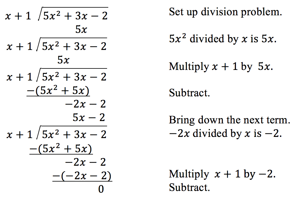
Divide [latex]5{x}^{2}+3x - 2[/latex] by [latex]x+1[/latex].
Divide [latex]16{x}^{3}-12{x}^{2}+20x - 3[/latex] by [latex]4x+5[/latex].
Watch the following video see an example of dividing polynomials with long division.
You can view the transcript for “Dividing polynomials using long division” here (opens in new window).
Using Synthetic Division to Divide Polynomials
The Main Idea
Synthetic division is a quicker way to divide polynomials when the divisor is a binomial with a leading coefficient of [latex]1[/latex]. It uses only the coefficients of the polynomials, simplifying the process significantly.
How to Use Synthetic Division
- Write the Opposite of k: If dividing by [latex]x-k[/latex], write down [latex]k[/latex].
- List the Coefficients: Write the coefficients of the polynomial you’re dividing.
- Bring Down the Leading Coefficient: This starts off your synthetic division.
- Multiply and Add: Multiply the leading coefficient by [latex]k[/latex], add it to the next coefficient, and continue this process.
- Find the Quotient and Remainder: The last number is the remainder, and the others form the coefficients of the quotient polynomial.


Watch the following video see an example of dividing polynomials using synthetic division.
You can view the transcript for “Synthetic Division of Polynomials” here (opens in new window).
Evaluate Polynomials
Evaluating a Polynomial Using the Remainder Theorem
The Main Idea
The Remainder Theorem is a quick way to evaluate polynomials. If you divide a polynomial [latex]f(x)[/latex]by [latex]x - k[/latex], the remainder is simply the value of [latex]f(k)[/latex]. It’s like a shortcut in a maze, allowing you to reach the end without going through all the paths.
For example, to evaluate [latex]f(x) = 6x^4 - x^3 - 15x^2 + 2x - 7[/latex] at [latex]x = 2[/latex], you can use synthetic division or directly substitute [latex]x[/latex] with [latex]2[/latex] to find the remainder.
Use the remainder theorem to evaluate [latex]f(x)=2x^5−3x^4−9x^3+8x^2+2[/latex] at [latex]x = -3[/latex].
Watch the following video for more on the remainder theorem.
You can view the transcript for “Remainder Theorem and Synthetic Division of Polynomials” here (opens in new window).
Using the Factor Theorem to Solve a Polynomial Equation
The Main Idea
The Factor Theorem is a bridge between zeros and factors of a polynomial. It states that a number [latex]k[/latex] is a zero of [latex]f(x)[/latex] if and only if [latex](x - k)[/latex] is a factor of [latex]f(x)[/latex]. This theorem is like a two-way street; knowing a zero lets you find a factor, and knowing a factor lets you find a zero.
For instance, to show that [latex](x + 2)[/latex] is a factor of [latex]x^3 - 6x^2 - x + 30[/latex], you can use synthetic division. If the remainder is zero, then [latex](x + 2)[/latex] is indeed a factor, and you can further factorize the quotient to find the remaining zeros of the polynomial.
Use the Factor Theorem to find the zeros of [latex]f(x)=x^3+4x^2−4x−16[/latex] given that [latex](x−2)[/latex] is a factor of the polynomial.
Zeros of Polynomial Functions
When we talk about the zeros of polynomial functions, we’re essentially looking for the values that make the polynomial equal to zero. These are the points where the graph of the polynomial will intersect the [latex]x[/latex]-axis. It’s like finding the roots of a tree that are hidden underground; they’re essential for the structure but not immediately visible.
Using the Rational Zero Theorem to Find Rational Zeros
The Main Idea
When we’re navigating the complex sea of polynomial functions, the Rational Zero Theorem is like our compass. It helps us pinpoint potential rational zeros using a simple yet powerful strategy: looking at the factors of the constant term and the leading coefficient.
For instance, consider a polynomial function that has zeros at [latex]\frac{2}{5}[/latex] and [latex]\frac{3}{4}[/latex]. These aren’t just numbers; they’re clues. By setting up equations with these zeros and constructing a quadratic function, we can see a pattern emerge. The numerators of these zeros ([latex]2[/latex] and [latex]3[/latex]) are factors of the constant term, while the denominators ([latex]5[/latex] and [latex]4[/latex]) are factors of the leading coefficient.
Quick Tips: Applying the Rational Zero Theorem
- List Out Factors: Start by listing all factors of the constant term and the leading coefficient of your polynomial.
- Form Ratios: Create all possible ratios [latex]\frac{p}{q}[/latex] where [latex]p[/latex] is a factor of the constant term and [latex]q[/latex] is a factor of the leading coefficient.
- Test Your Candidates: Evaluate each potential zero by plugging it into the polynomial. If the result is zero, you’ve found a true zero!
Use the Rational Zero Theorem to find the rational zeros of [latex]f(x) = 2x^3 + x^2 - 4x + 1[/latex].
Use the Rational Zero Theorem to find the rational zeros of [latex]f(x)=x^3−5x^2+2x+1[/latex].
Watch the following video see more on the rational zero theorem.
You can view the transcript for “Finding All Zeros of a Polynomial Function Using The Rational Zero Theorem” here (opens in new window).
Graphs of Polynomial Functions
Zeros and Multiplicity
The Main Idea
The zeros of a polynomial function are the points where the graph crosses the x-axis, meaning the output [latex]y[/latex] is zero. For example, the polynomial function [latex]f(x)=(x+3)(x−2)^2(x+1)^3[/latex]has zeros at:
- [latex]x = -3[/latex]
- [latex]x = 2[/latex]
- [latex]x = -1[/latex]
Quick Tips: Multiplicity and Graph Behavior
- Single Zeros: When a factor appears once, such as [latex]x+3[/latex], the graph crosses the [latex]x[/latex]-axis at this zero. This is a zero with multiplicity [latex]1[/latex].
- Even Multiplicity: Zeros with an even multiplicity, like [latex]x=2[/latex] in [latex](x−2)^2[/latex], indicate the graph touches the x-axis and turns around.
- Odd Multiplicity: Zeros with an odd multiplicity, such as [latex]x=−1[/latex] in [latex](x+1)^3[/latex], show that the graph will cross the [latex]x[/latex]-axis.
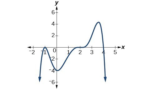
Use the graph of the function of degree [latex]5[/latex] to identify the zeros of the function and their multiplicities.
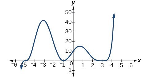
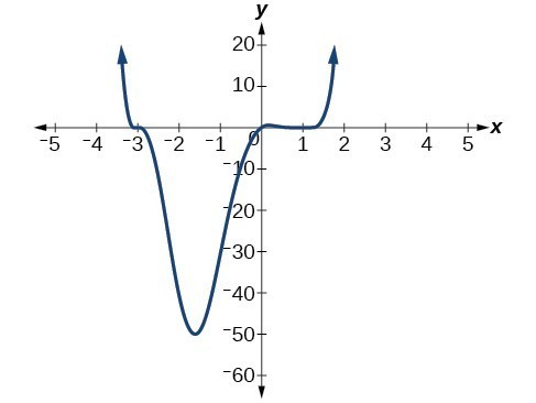
Use the graph below to find the zeros of the degree [latex]6[/latex] function and their multiplicities.

Watch the following video see an example of finding the zeros and their multiplicities.
You can view the transcript for “How to Determine the Multiplicity and Zeros of a Polynomial” here (opens in new window).
Determining the Number of Turning Points and Intercepts from the Degree of the Polynomial
The Main Idea
The number of turning points in a polynomial graph is related to the degree of the polynomial. A polynomial of degree [latex]n[/latex] can have up to [latex]n−1[/latex] turning points. For instance, a [latex]4[/latex]th-degree polynomial can have up to [latex]3[/latex] turning points. This is an essential concept in visualizing the shape of the graph.
The degree and leading coefficient of a polynomial function influence its end behavior. For a polynomial [latex]f(x)=ax^n[/latex]:
- If [latex]n[/latex] is odd and [latex]a>0[/latex], the ends of the graph go in opposite directions, with the right end going up.
- If [latex]n[/latex] is even and [latex]a>0[/latex], both ends of the graph go up.
This knowledge helps in sketching a rough graph of the polynomial function.
Without graphing the function, determine the maximum number of x-intercepts and turning points for [latex]f\left(x\right)=108 - 13{x}^{9}-8{x}^{4}+14{x}^{12}+2{x}^{3}[/latex].
The following video gives a 5 minute lesson on how to determine the number of intercepts and turning points of a polynomial function given its degree.
You can view the transcript for “Turning Points and X Intercepts of a Polynomial Function” here (opens in new window).
Identifying the Shape of the Graph of a Polynomial Function
Polynomial functions are like the diverse landscapes of mathematics, where each function can represent a unique terrain. The graphs of these functions are smooth and continuous, meaning they have no sharp turns or breaks. Just like a rolling hillside, these functions have a fluidity that’s both predictable and elegant.
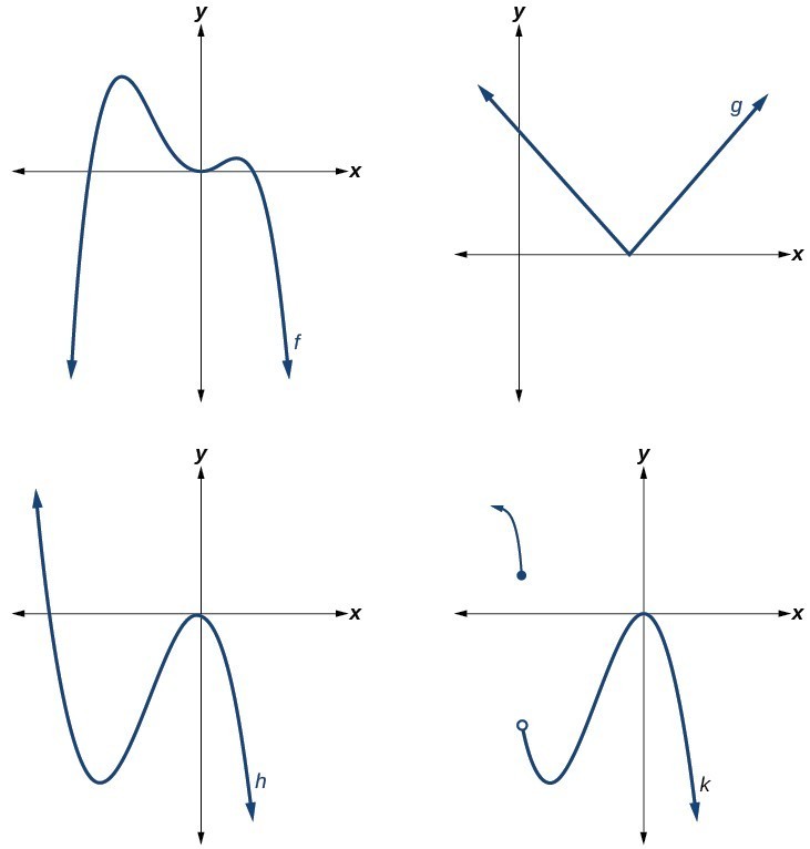
Which of the graphs below represents a polynomial function?
Identifying End Behavior of Polynomial Functions
The Main Idea
Quick Tips: Even vs. Odd Degree Polynomials
- Even Degree Polynomials: Think of even-degree polynomials like [latex]f(x)=x^2, g(x)=x^4,[/latex] and [latex]h(x)=x^6[/latex] as the serene hills that either rise or fall on both ends. As the degree increases, the middle part of the graph becomes flatter, and the ends become steeper, much like a valley becoming more pronounced with time.
- Odd Degree Polynomials: Odd-degree polynomials such as [latex]f(x)=x^3, g(x)=x^5,[/latex] and [latex]h(x)=x^7[/latex] are the adventurous mountain ranges of the polynomial world. One side ascends to the sky, while the other descends into the depths of the ocean. This is due to the fact that a negative input will yield a negative output when the degree is odd, creating a graph that has a perfect balance of ascent and descent.
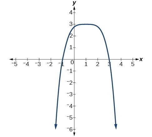
Describe the end behavior of the polynomial function in the graph below.
Given the function [latex]f\left(x\right)=0.2\left(x - 2\right)\left(x+1\right)\left(x - 5\right)[/latex], express the function as a polynomial in general form and determine the leading term, degree, and end behavior of the function.
In the following video, you’ll see more examples that summarize the end behavior of polynomial functions and which components of the function contribute to it.
You can view the transcript for “Summary of End Behavior or Long Run Behavior of Polynomial Functions” here (opens in new window).
The Sign of the Leading Term
The Main Idea
The leading term of a polynomial function is like the compass that dictates the direction of your graph. Changing the sign of this term is akin to entering a mirror world, where everything is flipped. Quick Tips: Even vs. Odd Degree Polynomials
- Positive Leading Term: When the leading term is positive, as in 3x^4[/latex], the arms of the graph reach for the heavens. The graph stays positive, no matter if [latex]x[/latex] is negative or positive.
- Negative Leading Term: Introduce a negative sign, and the graph of [latex]−3x^4[/latex] turns upside down, diving down as if reflecting in a lake. The negative leading term ensures that the arms of the polynomial are pointing downwards, regardless of the value of [latex]x[/latex].
The table below summarizes all four cases mentioned.
| Even Degree | Odd Degree |
|---|---|
 |
 |
 |
 |
Sketching Graphs
The Main Idea
When we sketch the graphs of polynomial functions, we’re essentially drawing a rough map of how the function behaves. It’s like sketching the path of a hiker in the mountains: we mark the starting point, the peaks, and the valleys. Here’s how we do it:
- Intercepts: These are our starting points. Just like a hiker checks a map for where to begin, we find where our graph crosses the axes.
- Symmetry: Is our path mirrored on either side? If our function is even, the graph is symmetric like butterfly wings across the [latex]y[/latex]-axis ([latex]f(−x)=f(x)[/latex]). If it’s odd, it’s like a twisty mountain road that flips across the origin ([latex]f(−x)=−f(x)[/latex]).
- Multiplicities and Intercepts: This tells us how our hiker approaches each peak or valley. Does she pass straight through, or does she hesitate and turn back a bit? The multiplicity of zeros gives us this behavior at [latex]x[/latex]-intercepts.
- End Behavior: This is the direction our hiker heads off into the distance. It’s determined by the leading term of our polynomial.
- Sketching the Graph: With all this information, we can draw a rough trail of our function, ensuring we don’t have more twists and turns (turning points) than the degree of the polynomial allows.
- Technology Check: Just like a hiker might check GPS, we can use graphing technology to confirm our path.
Watch the following video to see an example of sketching a polynomial.
You can view the transcript for “How to Sketch a Polynomial Function” here (opens in new window).
The following video is a bit long, but it covers how to graph a polynomial function using end behavior, multiplicity, and zeros.
You can view the transcript for “How To Graph Polynomial Functions Using End Behavior, Multiplicity & Zeros” here (opens in new window).
Writing Formulas for Polynomial Functions
The Main Idea
Writing the formula for a polynomial function from its graph is like retracing the hiker’s steps to map her exact route:
- [latex]X[/latex]-Intercepts: Find where the hiker started and finished her journey. These give us the factors of the polynomial.
- Multiplicity: How did she approach each peak? Did she go straight over, or did she pause and reflect? This tells us the multiplicity of each factor.
- Least Degree: We want the simplest map that still shows all the important points. Find the polynomial of the least degree that includes all factors.
- Stretch Factor: How steep were the mountains? Use another point (like the [latex]y[/latex]-intercept) to figure out the “stretch” of our polynomial, which scales the function up or down.
Given the graph below, write a formula for the function shown.
Watch the following video to see an example of writing the equation of a polynomial.
You can view the transcript for “Ex1: Find an Equation of a Degree 4 Polynomial Function From the Graph of the Function” here (opens in new window).