- Create and interpret equations of linear functions
- Use linear functions to model and draw conclusions from real-world problems
- Plot the graphs of linear equations
Point-Slope Form
Up until now, we have been using the slope-intercept form of a linear equation to describe linear functions. Now we will learn another way to write a linear function called point-slope form which is given below:
[latex]y-{y}_{1}=m\left(x-{x}_{1}\right)[/latex]
where [latex]m[/latex] is the slope of the linear function and [latex]({x}_{1},{y}_{1})[/latex] is any point which satisfies the linear function.
The point-slope form is derived from the slope formula.
[latex]\begin{array}{llll}{m}=\frac{y-{y}_{1}}{x-{x}_{1}}\hfill & \text{assuming }{ x }\ne {x}_{1}\hfill\\{ m }\left(x-{x}_{1}\right)=\frac{y-{y}_{1}}{x-{x}_{1}}\left(x-{x}_{1}\right)\hfill & \text{Multiply both sides by }\left(x-{x}_{1}\right)\hfill\\{ m }\left(x-{x}_{1}\right)=y-{y}_{1}\hfill & \text{Simplify}\hfill \\ y-{y}_{1}={ m }\left(x-{x}_{1}\right)\hfill &\text{Rearrange}\hfill \end{array}[/latex]
Keep in mind that slope-intercept form and point-slope form can be used to describe the same linear function. We can move from one form to another using basic algebra. For example, suppose we are given the equation [latex]y - 4=-\frac{1}{2}\left(x - 6\right)[/latex] which is in point-slope form. We can convert it to slope-intercept form as shown below.
[latex]\begin{array}{llll}y - 4=-\frac{1}{2}\left(x - 6\right)\hfill & \hfill \\ y - 4=-\frac{1}{2}x+3\hfill & \text{Distribute the }-\frac{1}{2}.\hfill \\ \text{}y=-\frac{1}{2}x+7\hfill & \text{Add 4 to each side}.\hfill \end{array}[/latex]
Therefore, the same line can be described in slope-intercept form as [latex]y=-\frac{1}{2}x+7[/latex].
point-slope form
Point-slope form of a linear equation takes the form
[latex]y-{y}_{1}=m\left(x-{x}_{1}\right)[/latex]
where [latex]m[/latex] is the slope and [latex]{x}_{1 }[/latex] and [latex]{y}_{1}[/latex] are the [latex]x[/latex] and [latex]y[/latex] coordinates of a specific point through which the line passes.
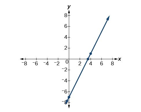
Point-slope form is particularly useful if we know one point and the slope of a line. For example, suppose we are told that a line has a slope of [latex]2[/latex] and passes through the point [latex]\left(4,1\right)[/latex]. We know that [latex]m=2[/latex] and that [latex]{x}_{1}=4[/latex] and [latex]{y}_{1}=1[/latex]. We can substitute these values into point-slope form.
[latex]\begin{array}{l}y-{y}_{1}=m\left(x-{x}_{1}\right)\\ y - 1=2\left(x - 4\right)\end{array}[/latex]
If we wanted to rewrite the equation in slope-intercept form, we apply algebraic techniques.
[latex]\begin{array}{llll} y - 1=2\left(x - 4\right)\hfill & \hfill \\ y - 1=2x - 8\hfill & \text{Distribute the }2.\hfill \\ \text{}y=2x - 7\hfill & \text{Add 1 to each side}.\hfill \end{array}[/latex]
Both equations [latex]y - 1=2\left(x - 4\right)[/latex] and [latex]y=2x - 7[/latex] describe the same line. The graph of the line can be seen below.