- Create and interpret equations of linear functions
- Use linear functions to model and draw conclusions from real-world problems
- Plot the graphs of linear equations
Point-Slope Form
The Main Idea
You’ve been using slope-intercept form, [latex]y=mx+b[/latex], to describe linear functions. But did you know there’s another superhero in town? Meet Point-Slope Form, [latex]y-{y}_{1}=m\left(x-{x}_{1}\right)[/latex], where [latex]m[/latex] is the slope and [latex]({x}_{1},{y}_{1})[/latex] is a point on the line. This form is a game-changer when you know a specific point and the slope but don’t have the [latex]y[/latex]-intercept.
You can convert between point-slope and slope-intercept forms using basic algebra.
To convert to slope-intercept form, distribute any constants and isolate [latex]y[/latex]
Both forms describe the same line, so choose the one that makes your life easier!
Watch the following video for a worked example of finding point-slope form and converting it to slope-intercept form.
You can view the transcript for “Writing an equation using point slope form given a point and slope” here (opens in new window).
Writing and Interpreting Equations of Linear Functions: Two Points, Graphs, and Real-World Applications
The Main Idea
You’ve learned that two points can define a line. But did you know that this is like having two pieces of a puzzle that reveal the entire picture? When you have two points, you can find the slope and then use point-slope form to find the equation of the line.
Sometimes, all you have is a graph. No worries! You can still find the equation of the line. Just pick two points on the graph and use them to find the slope. Then, use the slope and one point to write the equation in point-slope form.
Quick Tips
- Choose Wisely: Pick points that are easy to read on the graph.
- Y-Intercept: Look for where the line crosses the [latex]y[/latex]-axis; this is your [latex]y[/latex]-intercept [latex]b[/latex].
Linear functions are not just theoretical constructs; they’re practical tools. For example, if you’re starting a business, you can use a linear function to model your costs. The slope might represent the cost per item, and the y-intercept could be your fixed costs like rent.
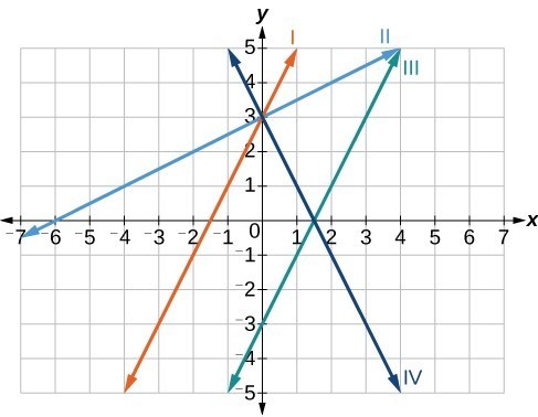
- [latex]f\left(x\right)=2x+3[/latex]
- [latex]g\left(x\right)=2x - 3[/latex]
- [latex]h\left(x\right)=-2x+3[/latex]
- [latex]j\left(x\right)=\frac{1}{2}x+3[/latex]

Watch the following video for more on writing point-slope and slope-intercept form from two points.
You can view the transcript for “Point-slope and slope-intercept form from two points | Algebra I | Khan Academy” here (opens in new window).
Watch the following video for more on writing the equation of a line from a graph.
You can view the transcript for “How To Find The Equation of a Line From a Graph | Algebra” here (opens in new window).
Building Linear Models
The Main Idea
Modeling Linear Functions Problem-Solving Strategy
- Identify changing quantities, and then define descriptive variables to represent those quantities. When appropriate, sketch a picture or define a coordinate system.
- Look for information that provides values for the variables or values for parts of the functional model, such as slope and initial value.
- Determine what we are trying to find, identify, solve, or interpret.
- Identify a solution pathway from the provided information to what we are trying to find. Often this will involve checking and tracking units, building a table, or even finding a formula for the function being used to model the problem.
- When needed, write a formula for the function.
- Solve or evaluate the function using the formula.
- Reflect on whether your answer is reasonable for the given situation and whether it makes sense mathematically.
- Clearly convey your result using appropriate units, and answer in full sentences when necessary.
You’ve probably heard the phrase “starting point” a lot, right? The [latex]y[/latex]-intercept is your starting point, and the slope guides you from there. Always remember, slope is your “rate of change,” and the [latex]y[/latex]-intercept is your “initial value.”
When given two points, use them to find your slope.
Diagrams are not just doodles; they’re visual aids. Use them to map out the problem and see the relationships between variables.
- Write a linear model to represent the cost [latex]C[/latex] of the company as a function of [latex]x[/latex], the number of doughnuts produced.
- Find and interpret the [latex]y[/latex]-intercept.
- Predict the population in 2014.
- Identify the year in which the population will reach [latex]54,000[/latex].
Graphing Linear Functions
The Main Idea
Graphing a Function by Plotting Points
Plotting Points: When graphing a function by plotting points, always choose at least two input values to get a minimum of two points on the graph. This helps you draw a more accurate line.
Plotting points is often the first method taught for graphing linear functions. But did you know that choosing three points can serve as a self-check? If all three don’t fall on the same line, you’ve likely made an error. So, next time you’re plotting points, go for that extra one; it’s like a built-in error detector!
Graphing a Linear Function Using y-intercept and Slope
Think of the [latex]y[/latex]-intercept and slope as the DNA of your graph. They uniquely identify how your graph will look. The [latex]y[/latex]-intercept tells you where the graph starts on the [latex]y[/latex]-axis, and the slope tells you how steep the line is. Knowing these two can save you time and effort in plotting multiple points.
Do all linear functions have [latex]y[/latex]-intercepts? Yes, they do, except for vertical lines, which aren’t functions. So, the next time you’re dealing with a linear function, you can be pretty confident that you’ll find a [latex]y[/latex]-intercept.
Graphing a Linear Function Using Transformations
You’ve learned that linear functions can be graphed using the slope-intercept form [latex]y=mx+b[/latex]. But did you know that you can also use transformations to graph these functions? Transformations like vertical stretches, compressions, and shifts can give you a new perspective on how linear functions behave.
Vertical Stretch/Compression: The coefficient [latex]f(x)=mx[/latex] acts as a vertical stretch or compression. If [latex]m>1[/latex], the graph stretches; if [latex]0 Vertical Shift: The constant [latex]b[/latex] in [latex]f(x)=mx+b[/latex] moves the graph up or down. Positive [latex]b[/latex] values shift the graph upwards, while negative [latex]b[/latex] values shift it downwards. When graphing using transformations, the order in which you apply them is crucial. For instance, if you have [latex]f(x)= \frac{1}{2}x−3[/latex], you should first apply the vertical compression by a factor of [latex]\frac{1}{2}[/latex] and then shift the graph down by [latex]3[/latex] units. This sequence aligns with the order of operations in mathematics, ensuring that you get an accurate graph.


Watch the following video for more on graphing linear functions using the slope and the [latex]y[/latex]-intercept.
You can view the transcript for “Graphing Linear Equations – Best Explanation” here (opens in new window).
Watch the following video for more on graphing linear functions with transformations.
You can view the transcript for “Graph a Linear Function as a Transformation of f(x)=x” here (opens in new window).