- Use the properties of logarithms to solve exponential models for time
- Identify the carrying capacity in a logistic growth model
- Use a logistic growth model to predict growth
Reversing an Exponent
Logarithms are mathematical tools that help us work with exponential models, particularly in solving for time or growth rates. They are the inverse of exponentials, meaning they ‘undo’ the exponential function.
Key Concepts:
- Common Logarithm: Denoted as [latex]log(x)[/latex], it is based on the exponential [latex]10^x[/latex] and is used to solve equations where the variable is an exponent.
- This means the statement [latex]10^{a} = b[/latex] is equivalent to the statement [latex]log(b) = a[/latex]
- Exponent property: [latex]\log\left({{A}^{r}}\right)=r\log\left(A\right)[/latex]
- Properties of Logarithms: These include product rule, quotient rule, power rule, and more, which are essential for simplifying and solving exponential equations.
To solve exponential equations with logarithms:
- Isolate the exponential. In other words, get it by itself on one side of the equation. This usually involves dividing by a number multiplying it.
- Take the log of both sides of the equation.
- Use the exponent property of logs to rewrite the exponential with the variable exponent multiplying the logarithm.
- Divide as needed to solve for the variable.
You can view the transcript for “Logarithms | Logarithms | Algebra II | Khan Academy” here (opens in new window).
You can view the transcript for “Logarithms – The Easy Way!” here (opens in new window).
Limits on Exponential Growth
In real-world situations, exponential growth often encounters limits, such as resource constraints or environmental factors. The logistic model adjusts the exponential growth formula to account for these limits, introducing the concept of carrying capacity.
Key Concepts:
- Carrying Capacity ([latex]K[/latex]): The maximum population or quantity that an environment can sustain.
- Adjusted Growth Rate: The growth rate in logistic models decreases as the population approaches the carrying capacity.
You can view the transcript for “Exponential Growth: a Commonsense Explanation.” here (opens in new window).
You can view the transcript for “Ecological Carrying Capacity-Biology” here (opens in new window).
Logistic Growth
The logistic model provides a framework for understanding growth in confined environments, such as population growth in a limited habitat or product adoption in a market.
The logistic growth model can be represented as [latex]P_n=P_{n-1}+r\left(1-\dfrac{P_{n-1}}{K}\right)P_{n-1}[/latex], where [latex]P_n[/latex] is the population at time [latex]n[/latex], [latex]r[/latex] is the growth rate, and [latex]K[/latex] is the carrying capacity.
This model can be applied to various scenarios, like predicting population of a specific type of animal in an environment or the spread of a technology in a market.
You can view the transcript for “Exponential vs Logistic Growth” here (opens in new window).
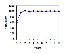
[latex]{{P}_{1}}={{P}_{0}}+1.50\left(1-\frac{{{P}_{0}}}{1000}\right){{P}_{0}}=600+1.50\left(1-\frac{600}{1000}\right)600=960[/latex]
[latex]{{P}_{2}}={{P}_{1}}+1.50\left(1-\frac{{{P}_{1}}}{1000}\right){{P}_{1}}=960+1.50\left(1-\frac{960}{1000}\right)960=1018[/latex]
Interestingly, even though the factor that limits the growth rate slowed the growth a lot, the population still overshot the carrying capacity. We would expect the population to decline the next year.
[latex]{{P}_{3}}={{P}_{2}}+1.50\left(1-\frac{{{P}_{3}}}{1000}\right){{P}_{3}}=1018+1.50\left(1-\frac{1018}{1000}\right)1018=991[/latex]
Calculating out a few more years and plotting the results, we see the population wavers above and below the carrying capacity, but eventually settles down, leaving a steady population near the carrying capacity.
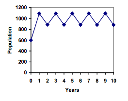
While it would be tempting to treat this only as a strange side effect of mathematics, this has actually been observed in nature. Researchers from the University of California observed a stable 2-cycle in a lizard population in California.[1]Taking this even further, we get more and more extreme behaviors as the growth rate increases higher. It is possible to get stable 4-cycles, 8-cycles, and higher. Quickly, though, the behavior approaches chaos (remember the movie Jurassic Park?).

All of the lizard island examples are discussed in this video.
You can view the transcript for “Logistic growth of lizards” here (opens in new window).