- Solve direct variation problems.
- Solve inverse variation problems.
- Solve problems involving joint variation.
Direct Variation
Direct variation is a fundamental concept in algebra that describes a linear relationship between two variables. In direct variation, one variable is a constant multiple of another. This concept is often used in real-world situations where two quantities vary in a consistent manner.
direct variation
If [latex]x[/latex] and [latex]y[/latex] are related by an equation of the form
[latex]y=k{x}^{n}[/latex]
then we say that the relationship is direct variation and [latex]y[/latex] varies directly with the [latex]n[/latex]th power of [latex]x[/latex].
- In direct variation relationships, there is a nonzero constant ratio [latex]k=\dfrac{y}{{x}^{n}}[/latex], where [latex]k[/latex] is called the constant of variation, which help defines the relationship between the variables.
[latex]\\[/latex]
Nicole’s earnings can be found by multiplying her sales by her commission. The formula [latex]e = 0.16s[/latex] tells us her earnings, [latex]e[/latex], come from the product of [latex]0.16[/latex], her commission, and the sale price of the vehicle, [latex]s[/latex].
[latex]\\[/latex]
If we create a table, we observe that as the sales price increases, the earnings increase as well, which should be intuitive.
| [latex]s[/latex], sales prices | [latex]e = 0.16s[/latex] | Interpretation |
|---|---|---|
| [latex]$4,600[/latex] | [latex]e=0.16(4,600)=736[/latex] | A sale of a [latex]$4,600[/latex] vehicle results in [latex]$736[/latex] earnings. |
| [latex]$9,200[/latex] | [latex]e=0.16(9,200)=1,472[/latex] | A sale of a [latex]$9,200[/latex] vehicle results in [latex]$1472[/latex] earnings. |
| [latex]$18,400[/latex] | [latex]e=0.16(18,400)=2,944[/latex] | A sale of a [latex]$18,400[/latex] vehicle results in [latex]$2944[/latex] earnings. |
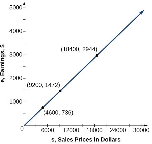
Notice that earnings are a multiple of sales. As sales increase, earnings increase in a predictable way. Double the sales of the vehicle from [latex]$4,600[/latex] to [latex]$9,200[/latex], and we double the earnings from [latex]$736[/latex] to [latex]$1,472[/latex].
As the input increases, the output increases as a multiple of the input. A relationship in which one quantity is a constant multiplied by another quantity is called direct variation. Each variable in this type of relationship varies directly with the other.
- Identify the input, [latex]x[/latex], and the output, [latex]y[/latex].
- Determine the constant of variation. You may need to divide [latex]y[/latex] by the specified power of [latex]x[/latex] to determine the constant of variation.
- Use the constant of variation to write an equation for the relationship.
- Substitute known values into the equation to find the unknown.
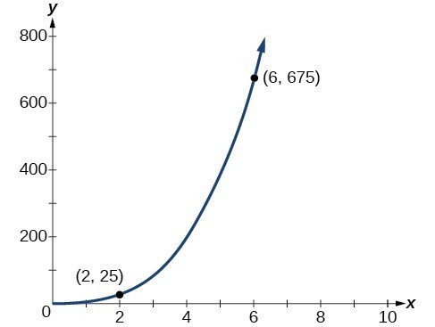
No. Direct variation equations are power functions—they may be linear, quadratic, cubic, quartic, radical, etc. But all of the graphs pass through [latex](0, 0)[/latex].